Welcome to 3D Slicer’s documentation!

This is documentation is a work in progress, in preparation for the new Slicer-5.0 release.

For Slicer-4.10 documentation, refer to the 3D Slicer wiki.

About 3D Slicer

What is 3D Slicer?

• A software application for visualization and analysis of medical image computing data sets. All commonly used data sets are supported, such as images, segmentations, surfaces, annotations, transformations, etc., in 2D, 3D, and 4D. Visualization is available on desktop and in virtual reality. Analysis includes segmentation, registration, and various quantifications.
• A research software platform, which allows researchers to quickly develop and evaluate new methods and distribute them to clinical users. All features are available and extensible in Python and C++. A full Python environment is provided where any Python packages can be installed and combined with built-in features. Slicer has a built-in Python console and can act as a Jupyter notebook kernel with remote 3D rendering capabilities.
• Product development platform, which allows companies to quickly prototype and release products to users. Developers can focus on developing new methods and do not need to spend time with redeveloping basic data import/export, visualization, interaction features. The application is designed to be highly customizable (with custom branding, simplified user interface, etc.). 3D Slicer is completely free and there are no restrictions on how it is used - it is up to the software distributor to ensure that the developed application is suitable for the intended use.

Note: There is no restriction on use, but Slicer is NOT approved for clinical use and the distributed application is intended for research use. Permissions and compliance with applicable rules are the responsibility of the user. For details on the license see here.

Highlights:

• Free, open-source software available on multiple operating systems: Linux, macOS and Windows.
• Multi organ: from head to toe.
• Support for multi-modality imaging including, MRI, CT, US, nuclear medicine, and microscopy.
• Real-time interface for medical devices, such as surgical navigation systems, imaging systems, robotic devices, and sensors.
• Highly extensible: users can easily add more capabilities by installing additional modules from the Extensions manager, running custom Python scripts in the built-in Python console, run any executables from the application’s user interface, or implement custom modules in Python or C++.
• Large and active user community.

License

The 3D Slicer software is distributed under a BSD-style open source license that is compatible with the Open Source Definition by The Open Source Initiative and contains no restrictions on use of the software.

To use Slicer, please read the 3D Slicer Software License Agreement before downloading any binary releases of the Slicer.

How to cite

3D Slicer as a platform

To acknowledge 3D Slicer as a platform, please cite the Slicer web site and the following publications when publishing work that uses or incorporates 3D Slicer:

Fedorov A., Beichel R., Kalpathy-Cramer J., Finet J., Fillion-Robin J-C., Pujol S., Bauer C., Jennings D., Fennessy F.M., Sonka M., Buatti J., Aylward S.R., Miller J.V., Pieper S., Kikinis R. 3D Slicer as an Image Computing Platform for the Quantitative Imaging Network. Magn Reson Imaging. 2012 Nov;30(9):1323-41. PMID: 22770690. PMCID: PMC3466397.

Individual modules

To acknowledge individual modules: each module has an acknowledgment tab in the top section. Information about contributors and funding source can be found there:

Additional information (including information about the underlying publications) can be typically found on the manual pages accessible through the help tab in the top section:

Acknowledgments

Slicer is made possible through contributions from an international community of scientists from a multitude of fields, including engineering and biomedicine. The following sections give credit to some of the major contributors to the 3D Slicer core effort. Each 3D Slicer extension has a separate acknowledgements page with information specific to that extension.

Ongoing Slicer support depends on YOU

Please give the Slicer repository a star on github. This is an easy way to show thanks and it can help us qualify for useful services that are only open to widely recognized open projects. Don’t forget to cite our publications because that helps us get new grant funding. If you find Slicer is helpful like the community please get involved. You don’t need to be a programmer to help!

Major Contributors

• Ron Kikinis: Principal Investigator
• Steve Pieper: Chief Architect
• Jean-Christophe Fillion-Robin: Lead Developer
• Nicole Aucoin
• Stephen Aylward
• Andrey Fedorov
• Noby Hata
• Hans Johnson
• Tina Kapur
• Gabor Fichtinger
• Andras Lasso
• Csaba Pinter
• Jim Miller
• Sonia Pujol: Director of Training
• Junichi Tokuda
• Lauren O’Donnell
• Andinet Enquobahrie
• Beatriz Paniagua

Contributors are not only developers, but also individual helping to secure funding and move the platform forward.

Groups Contributing to the Core Engineering of Slicer in a Major Way

• SPL: Ron Kikinis, Nicole Aucoin, Lauren O’Donnell, Andrey Fedorov, Isaiah Norton, Sonia Pujol, Noby Hata, Junichi Tokuda
• Isomics: Steve Pieper, Alex Yarmarkovich
• Kitware: Jean-Christophe Fillion-Robin, Julien Finet, Will Schroeder, Stephen Aylward, Andinet Enquobahrie, Beatriz Paniagua, Matt McCormick, Johan Andruejol, Max Smolens, Alexis Girault, Sam Horvath
• University of Iowa: Hans Johnson
• GE: Jim Miller
• Perk Lab, Queen’s University: Andras Lasso, Tamas Ungi, Csaba Pinter, Gabor Fichtinger
• Kapteyn Astronomical Institute, University of Groningen: Davide Punzo

Funding Sources

Many of the activities around the Slicer effort are made possible through funding from public and private sources. The National Institutes of Health of the USA is a major contributor through a variety of competitive grants and contracts.

See a selection of funding grants here.

Commercial Use

We invite commercial entities to use 3D Slicer.

Slicer’s License makes Commercial Use Available

• 3D Slicer is a Free Open Source Software distributed under a BSD style license.
• The license does not impose restrictions on the use of the software.
• 3D Slicer is NOT FDA approved. It is the users responsibility to ensure compliance with applicable rules and regulations.
• For details, please see the 3D Slicer Software License Agreement.

Commercial Partners

• Ebatinca SL is an international technology company in Las Palmas, Spain focused on technology for sustainable development.
• Isomics uses 3D Slicer in a variety of academic and commercial research partnerships in fields such as planning and guidance for neurosurgery, quantitative imaging for clinical trials, clinical image informatics.
• Kitware Integral to continuing to support the 3D Slicer community, Kitware is also offering consulting services in response to the rapidly growing demand for the development of proprietary applications and commercial products based on 3D Slicer. Kitware has used 3D Slicer to rapidly prototype solutions in nearly every aspect of medical imaging and is also collaborating on the development of commercial pre-clinical and clinical products based on 3D Slicer.
• Pixel Medical builds on and contributes to 3D Slicer to develop innovative medical software from idea to clinical prototype to finished product, and to support academic research projects. Areas of expertise include radiation therapy, image guided therapy, virtual & augmented reality, hardware & device support, and machine learning & artificial intelligence.

Listed in alphabetical order.

3D Slicer based products

Many companies prefer not to disclose what software components they use in their products, therefore here we can only list a few commercial products that are based on 3D Slicer:

• Allen Institute for Brain Science: Cell Locator, Desktop application for manually aligning specimens to annotated 3D spaces.
• Radiopharmaceutical Imaging and Dosimetry: RPTDose, a 3D Slicer-based application that streamlines and integrates quantitative imaging analysis and dose estimation techniques to guide and optimize the use of radiopharmaceutical therapy agents in clinical trials. See more information on this Kitware blog.
• SonoVol is developing a whole-body ultrasound imaging system for small animals. This start-up company arose from research in the Department of Biomedical Engineering at the University of North Carolina at Chapel Hill. See more information on this Kitware blog.
• Xoran Technologies: Image-guided Platform for Deep Brain Stimulation Surgery 1. See more information on this Kitware blog.
• Xstrahl is developing a Small Animal Radiation Research Platform (SARRP) that uses 3D Slicer as its front-end application for radiation therapy beam placement and system control. See more information on this Kitware blog.

Listed in alphabetical order.

Contact us

It is recommended to post any questions, bug reports, or enhancement requests to the Slicer forum.

Our online issue tracker is available here.

For commercial/confidential consulting, contact one of the commercial partners.

Getting Started

Welcome to the 3D Slicer community. This page contains information that you need to get started with 3D Slicer, including how to install and use basic features and where to find more information.

System requirements

3D Slicer runs on any Windows, Mac, or Linux computer that was released in the last 5 years. Older computers may work (depending mainly on graphics capabilites). Slicer can also run on virtual machines and docker containers.

Operating system versions

• Windows: Windows 10, with all recommended updates installed. Windows 10 Version 1903 (May 2019 Update) version is required for support of international characters (UTF-8) in filenames and text. Microsoft does not support Windows 8.1 and Windows 7 anymore and Slicer is not tested on these legacy operating system versions, but may still work.
• macOS: macOS High Sierra (10.13) or later. Latest public release is recommended.
• Linux: Ubuntu 18.04 or later
  CentOS 7 or later. Latest LTS (Long-term-support) version is recommended.

Recommended hardware configuration

• Memory: more than 4GB (8 or more is recommended). As a general rule, have 10x more memory than the amount of data that you load.
• Display: a minimum resolution of 1024 by 768 (1280 by 1024 or better is recommended).
• Graphics: Dedicated graphics hardware (discrete GPU) memory is recommended for fast volume rendering. GPU: Graphics must support minimum OpenGL 3.2. Integrated graphics card is sufficient for basic visualization. Discrete graphics card (such as NVidia GPU) is recommended for interactive 3D volume rendering and fast rendering of complex scenes. GPU texture memory (VRAM) should be larger than your largest dataset (e.g., working with 2GB data, get VRAM > 4GB) and check that your images fit in maximum texture dimensions of your GPU hardware. Except rendering, most calculations are performed on CPU, therefore having a faster GPU will generally not impact the overall speed of the application.
• Some computations in 3D Slicer are multi-threaded and will benefit from multi core, multi CPU configurations.
• Interface device: a three button mouse with scroll wheel is recommended. Pen, multi-touchscreen, touchpad, and graphic tablet are supported. All OpenVR-compatible virtual reality headsets are supported for virtual reality display.
• Internet connection to access extensions, Python packages, online documentation, sample data sets, and tutorials.

Installing 3D Slicer

To download Slicer, click here.

Notes:

• The “Preview Release” of 3D Slicer is updated daily (process starts at 11pm ET and takes few hours to complete) and represents the latest development including new features and fixes.
• The “Stable Release” is usually updated a few times a year and is more rigorously tested.
• Slicer is generally simple to install on all platforms. It is possible to install multiple versions of the application on the same user account and they will not interfere with each other. If you run into mysterious problems with your installation you can try deleting the application settings files.
• Only 64-bit Slicer installers are available to download. Developers can attempt to build 32-bit versions on their own if they need to run Slicer on a 32-bit operating system. That said, this should be carefully considered as many clinical research tasks, such as processing of large CT or MR volumetric datasets, require more memory than can be accommodated with a 32-bit program.

Once downloaded, follow the instructions below to complete installation:

Windows

• Run the installer.
  • Current limitation: Installation path must only contain English (ASCII printable) characters because otherwise some Python packages may not load correctly (see this issue for more details).
• Run Slicer from the Windows start menu
• Use “Apps & features” in Windows settings to remove the application

Mac

• Drag the Slicer application (Slicer.app) to your Applications folder or other location of your choice.
• You cannot install extensions into the read-only volume so you must copy before installing extensions.
• Delete the Slicer.app folder to uninstall

Installing Preview Release: Currently, preview release packages are not signed. Therefore, when the application is started the first time the following message is displayed: “Slicer… can’t be opened because it is from an unidentified developer”. To resolve this error, locate the application in Finder and right-click (two-finger click) and click Open. When it says This app can’t be opened go ahead and hit cancel. Right click again and say Open (yes, you need to repeat the same as you did before - the outcome will be different than the first time). Click the Open (or Open anyway) button to start the application. See more explanation and alternative techniques here.

Linux

• Open the tar.gz archive and copy directory to the location of your choice. Run the Slicer executable.
• Remove the directory to uninstall

Note: Slicer is expected to work on the vast majority of desktop and server Linux distributions. The system is required to provide at least GLIBC 2.17 and GLIBCCC 3.4.19. For more details, read here.

Debian / Ubuntu

The following may be needed on fresh debian or ubuntu:

sudo apt-get install libpulse-dev libnss3 libglu1-mesa
sudo apt-get install --reinstall libxcb-xinerama0

To run Slicer-4.11-2020-09-30 on older debian (e.g. debian 9) you may also need:

sudo apt-get install libxcb-icccm4-dev libxcb-image0-dev libxcb-keysyms1-dev libxcb-randr0 libxcb-render-util0 libxcb-xkb-dev libxkbcommon-x11-dev

ArchLinux

ArchLinux runs the strip utility by default; this needs to be disabled in order to run Slicer binaries. For more information see this thread on the Slicer Forum.

Fedora

Install the dependencies:

sudo dnf install mesa-libGLU libnsl

The included libcrypto.so.1.1 in Slicer-4.11 is incompatible with the system libraries used by Fedora 35. The fix, until it is updated, is to move/remove the included libcrypto files:

$SLICER_ROOT/lib/Slicer-4.11/libcrypto.*

Using Slicer

3D Slicer offers lots of features and gives users great flexibility in how to use them. As a result, new users may be overwhelmed with the number of options and have difficulty figuring out how to perform even simple operations. This is normal and many users successfully crossed this difficult stage by investing some time into learning how to use this software.

How to learn Slicer?

Quick start

You may try to figure out how the application works by loading data sets and explore what you can do.

Load data

Open 3D Slicer and using the Welcome panel either load your own data or download sample data to explore. Sample data is often useful for trying the features of 3D Slicer if you don’t have data of your own.

View data

Data module’s Subject hierarchy tab shows all data sets in the scene. Click the “eye” icon to show/hide an item in all views.

You can customize views (show orientation marker, ruler, change orientation, transparency) by clicking on the push pin in the top left corner of viewer. In the slice viewers, the horizontal bar can be used to scroll through slices or select a slice.

Process data

3D Slicer is built on a modular architecture. Choose a module to process or analyze your data. Most important modules are the followings (complete list is available in Modules section):

• Welcome: The default module when 3D Slicer is started. The panel features options for loading data and customizing 3D Slicer. Below those options are drop-down boxes that contain essential information for using 3D Slicer.
• Data: acts as a central data-organizing hub. Lists all data currently in the scene and allows basic operations such as search, rename, delete and move.
• DICOM: Import and export DICOM objects, such as images, segmentations, strucutre sets, radiation therapy objects, etc.
• Volumes: Used for changing the appearance of various volume types.
• Volume Rendering: Provides interactive visualization of 3D image data.
• Segmentations: Edit display properties and import/export segmentations.
• Segment Editor: Segment 3D volumes using various manual, semi-automatic, and automatic tools.
• Markups: Allows the creation and editing of markups associated with a scene. Currently, lists of fiducially are supported as markups.
• Models: Loads and adjusts display parameters of models. Allows the user to change the appearance of and organize 3D surface models.
• Transforms: This module is used for creating and editing transformation matrices. You can establish these relations by moving nodes from the Transformable list to the Transformed list or by dragging the nodes under the Transformation nodes in the Data module.

Save data

Data sets loaded into the application can be saved using Save data dialog or exported to DICOM format using DICOM module. Detailes are described in Data loading and saving section.

Extensions

3D Slicer supports plug-ins that are called extensions. An extension could be seen as a delivery package bundling together one or more Slicer modules. After installing an extension, the associated modules will be presented to the user as built-in ones. Extensions can be downloaded from the extensions manager to selectively install features that are useful for the end-user.

For details about downloading extensions, see Extensions Manager documentation. Click here for a full list of extensions. The links on the page will provide documentation for each extension.

Slicer is extensible. If you are interested in customizing or adding functionality to Slicer, click here.

Tutorials

You learn both basic concepts and highly specialized workflows from the numerous available step-by-step and video tutorials.

Try the Welcome Tutorial and the Data Loading and 3D Visualization Tutorial to learn the basics.

For more tutorials, visit the Tutorial page.

User manual

Browse the User Guide section to find quick overview of the application user interface or Modules section for detailed description of each module.

Ask for help

3D Slicer has been around for many years and many questions have been asked and answered about it already. If you have any questions, then you may start with a web search, for example Google slicer load jpg to find out how you can import a stack of jpg images.

The application has a large and very friendly and helpful user community. We have poeple who will happy to help with simple questions, such as how to do a specific task in Slicer, and we have a large number of engineering and medical experts who can give you advice with how to solve complex problems.

If you have any questions, go to the Slicer forum and ask us!

Get Help

Contact the Slicer community or commercial partners if you have any questions, bug reports, or enhancement requests - following the guidelines described below.

I need help in using Slicer

• You can start with typing your question into Google web search. There is a good chance that your question has been asked and answered before and all questions ever asked about Slicer are publicly available and indexed by Google. Most up-to-date information sources are the Slicer forum and Slicer documentation on read-the-docs. Google may find older discussions on former Slicer mailing lists and wiki pages, which may or may not be exactly accurate for the current version of Slicer, but may still provide useful hints.
• Try your best to sort out the issue by reading documentation, portfolio of training materials, and checking error logs (in application menu bar: View->Error log).
• If you are still unclear about what to do: ask a question on the Slicer Forum. In addition to describing the specific question, it helps if you describe the context of your question (who you are, what you are working on, why it is important, what is the overall goal of your project). Knowing more about you and your project increases the chance that somebody volunteers to answer the question and you may get a more relevant answer.

I want to report a problem

If something is definitely not working as intended then file a bug report in the Slicer issue tracker.

It is important to provide enough specific information so that a software developer can duplicate the problem. Follow instructions in the bug report template.

If the problem occurs by using the application from custom code, follow SSCCE (Short, Self Contained, Correct, Example) approach.

Don’t be anonymous: real people trying hard to solve real problems are more likely to get valuable help. If you tell about yourself and your project then it may get more attention.

I would like to request enhancement or new feature

First search on the Slicer forum to see if someone asked for this feature already. If you find a very similar request, tell us that you are interested in it too.

If you cannot find a similar topic on the Slicer forum, write a post in the Feature request category

If you write about yourself and your project then there is a higher chance that your request will be worked on. Describe what assistance you can offer for the implementation (your own time, funding, etc.).

I would like to let the Slicer community know, how Slicer helped me in my research

Please send us the citation for your paper posting in Community category in Slicer forum.

Background: Funding for Slicer is provided through competitive mechanisms primarily by the United States government and to a lesser extent through funding from other governments. The justification for those resources is that Slicer enables scientific work. Knowing about scientific publications enabled by Slicer is a critical step in this process. Given the international nature of the Slicer community, the nationality of the scientists is not important. Every good paper counts.

Troubleshooting

Slicer application does not start

• Your computer CPU or graphics capabilities may not meet minimum system requirements. Updating your graphics driver may fix some problems, but if that does not help and you have an old computer then you may need to upgrade to a more recently manufactured computer.
• Slicer may not work if it is installed in a folder that has special characters in their name. Try installing Slicer in a path that only contains latin letters and numbers (a-z, 0-9).
• Your Slicer settings might have become corrupted
  • Try launching slicer using Slicer.exe --disable-settings (if it fixes the problem, delete Slicer.ini and Slicer-.ini files from your Slicer settings directory.
  • Rename or remove your Slicer settings directory (for example, c:\Users\<yourusername>\AppData\Roaming\NA-MIC). See instructions for getting the settings directory here. Try to launch Slicer.
• There may be conflicting/incompatible libraries in your system path (most likely caused by installing applications that place libraries in incorrect location on your system). Check your system logs for details and report the problem.
  • On Windows:
    • Start Event Viewer (eventvwr.exe), select Windows Logs / Application, and find the application error. If there is a DLL loading problem a line similar to this will appear: Faulting module path: <something>.dll. If you found a line similar to this, then try the following workaround: Start a command window. Enter set path= to clear the path variable. Enter Slicer.exe to start Slicer. If Slicer starts successfully then you need to remove remove unnecessary items from the system path (or delete the libraries installed at incorrect locations).
    • If Slicer still does not work then collect some more information and report the problem:
      • Get DLL dependency information using Dependency Walker tool:
        • Download depends.exe from here
        • Run depends.exe using the Slicer launcher: Slicer.exe --launch path\to\depends.exe "bin\SlicerApp-real.exe"
        • In dependency walker: Make sure the full path of DLLs are shown (click View / Full paths if you only see the DLL names). Use File / Save as… => Comma Separated Values (*.csv) to save logs to a file.
      • Enable process loading logging using the sxstrace tool, start Slicer, and save the log file (see instructions here)

User Interface

Application overview

Slicer stores all loaded data in a data repository, called the “scene” (or Slicer scene or MRML scene). Each data set, such as an image volume, surface model, or point set, is represented in the scene as a “node”.

Slicer provides a large number “modules”, each implementing a specific set of functions for creating or manipulating data in the scene. Modules typically do not interact with each other directly: they just all operate on the data nodes in the scene. Slicer package contains over 100 built-in modules and additional modules can be installed by using the Extensions Manager.

Module Panel

This panel (located by default on the left side of the application main window) displays all the options and features that the current module offers to the user. Current module can be selected using the Module Selection toolbar.

Data Probe is located at the bottom of the module panel. It displays information about view content at the position of the mouse pointer.

Views

Slicer displays data in various views. The user can choose between a number of predefined layouts, which may contain slice, 3D, chart, and table views.

The Layout Toolbar provides a drop-down menu of layouts useful for many types of studies. When Slicer is exited normally, the selected layout is saved and restored next time the application is started.

Application Menu

• File: Functions for loading a previouly saved scene or individual datasets of various types, and for downloading sample datasets from the internet. An option for saving scenes and data is also provided here. Add Data allows loading data from files. DICOM module is recommended to import data from DICOM files and loading of imported DICOM data. Save opens the “Save Data” window, which offers a variety of options for saving all data or selected datasets.
• Edit: Contains an option for showing Application Settings, which allows users to customize appearance and behavior of Slicer, such as modules displayed in the toolbar, application font size, temporary directory location, location of additional Slicer modules to include.
• View: Functions for showing/hiding additional windows and widgets, such as Extensions Manager for installing extensions from Slicer app store, Error Log for checking if the application encountered any potential errors, Python Interactor for getting a Python console to interact with the loaded data or modules, show/hide toolbars, or switch view layout.

Toolbar

Toolbar provides quick access to commonly used functions. Individual toolbar panels can be shown/hidden using menu: View / Toolbars section.

Module Selection toolbar is used for selecting the currently active “module”. The toolbar provides options for searching for module names (Ctrl + f or click on magnify glass icon) or selecting from a menu. Module history dropdown button shows the list of recently used modules. Arrow buttons can be used for going back to/returning from previously used module.

Favorite modules toolbar contains a list of most frequently used modules. The list can be customized using menu: Edit / Application settings / Modules / Favorite Modules. Drag-and-drop modules from the Modules list to the Favorite Modules list to add a module.

Status bar

This panel may display application status, such as current operation in progress. Clicking the little X icons displays the Error Log window.

Review loaded data

Data available in Slicer can be reviewed in the Data module, which can be found on the toolbar or the modules list . More details about the module can be found on the Slicer wiki.

The Data module’s default Subject hierarchy tab can show the datasets in a tree hierarchy, arranged as patient/study/series as typical in DICOM, or any other folder structure:

The Subject hierarchy view contains numerous built-in functions for all types of data. These functions can be accessed by right-clicking the node in the tree. The list of actions differs for each data type, so it is useful to explore the options.

Medical imaging data comes in various forms and representations, which may confuse people just starting in the field. The following diagram gives a brief overview about the most typical data types encountered when using Slicer, especially in a workflow that involves segmentation.

Selecting displayed data

Data module’s Subject hierarchy tab shows all data sets in the scene. Click the “eye” icon to show/hide an item in all views. Drag-and-drop an item into a view to show it in that view.

Multiple items can be selected in the subject hierarchy tree using Ctrl-Left-Click or Shift-Left-Click and dragged at once into selected view. If two volumes are dragged into a view at the same time then they will be both shown, blended together.

If a view is displayed only in selected views, you can right-click on the item and select “Show in all views” to quickly show in all views.

If view link is enabled for a slice view then dragging a volume to any of the views will show the volume in all the views in that group.

Interacting with views

View Cross-Reference

Holding down the Shift key while moving the mouse in any slice or 3D view will cause the Crosshair to move to the selected position in all views. By default, when the Crosshair is moved in any views, all slice views are scrolled to the same RAS position indexed by the mouse. This feature is useful when inspecting.

To show/hide the Crosshair position, click crosshair icon .

To customize behavior and appearance of the Crosshair, click the “down arrow” button on the right side of the crosshair icon.

Mouse Modes

Slicer has multiple mouse modes: Transform (which allows interactive rotate, translate and zoom operations), Window/Level to adjust brightness/contrast of the image volumes, and Place (which permits objects to be interactively placed in slice and 3D views).

The toolbar icons that switch between these mouse modes are shown from left to right above, respectively. Place Fiducial is the default place option as shown above; options to place other nodes such as Ruler and Region of Interest Widgets are also available from the drop-down Place Mode menu.

Note: Transform mode is the default interaction mode. By default, Place mode persists for one “place” operation after the Place Mode icon is selected, and then the mode switches back to Transform. Place mode can be made persistent (useful for creating multiple fiducial points, rulers, etc.) by checking the Persistent checkbox shown rightmost in the Mouse Mode Toolbar.

Adjusting image window/level

Medical images typically contain thousands of gray levels, but regular computer displays can display only 256 gray levels, and the human eye also has limitation in what minimum contrast difference it can notice (see Kimpe 2007 for more specific information). Therefore, medical images are displayed with adjustable brightness/contrast (window/level).

By default 3D Slicer uses window/level setting that is specified in the DICOM file. If it is not available then window/level is set so that the entire intensity range of the image (except top/bottom 0.1%, to not let a very thin tail of the intensity distribution to decrease the image contrast too much).

Window/level can be manually adjusted anytime by clicking on “Adjust window/level” button on the toolbar then left-click-and-drag in any of the slice viewers. Optimal window/level can be computed for a chosen area by lef-click-and-dragging while holding down Ctrl key.

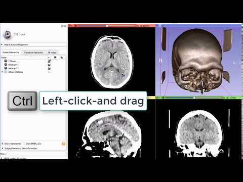
Additional window/level options, presets, intensity histogram, automatic adjustments are available in Display section of Volumes module.

3D View

Displays a rendered 3D view of the scene along with visual references to specify orientation and scale.

Default orientation axes: A = anterior, P = posterior, R = right, L = left, S = superior and I = inferior.

3D View Controls: The blue bar across any 3D View shows a pushpin icon on its left. When the mouse rolls over this icon, a panel for configuring the 3D View is displayed. The panel is hidden when the mouse moves away. For persistent display of this panel, just click the pushpin icon.

Slice View

Three default slice views are provided (with Red, Yellow and Green colored bars) in which Axial, Saggital, Coronal or Oblique 2D slices of volume images can be displayed. Additional generic slice views have a grey colored bar and an identifying number in their upper left corner.

Slice View Controls: The colored bar across any slice view shows a pushpin icon on its left (Show view controls). When the mouse rolls over this icon, a panel for configuring the slice view is displayed. The panel is hidden when the mouse moves away. For persistent display of this panel, just click the pushpin icon. For more options, click the double-arrow icon (Show all options).

View Controllers module provides an alternate way of displaying these controllers in the Module Panel.

• Reset field of view (small square) centers the slice on the current background volume
• Show in 3D “eye” button in the top row can show the current slice in 3D views. Drop-down menu of the button contains advanced options to customize how this slice is rendered: “…match volume” means that the properties are taken from the full volume, while “…match 2D” means that the properties are copied from the current slice view (for example, copies zoom and pan position). Typically these differences are subtle and the settings can be left at default.
• Slice orientation displays allows you to choose the orientation for this slice view.
• Lightbox to select a mosiac (a.k.a. contact sheet) view. Not all operations work in this mode and it may be removed in the future.
• Reformat allows interactive manipulation of the slice orientation.
• Slice offset slider allows slicing through the volume. Step size is set to the background volume’s spacing by default but can be modified by clicking on “Spacing and field of view” button.
• Blending mode specifies how foreground and background layers are mixed.
• Spacing and field of view Spacing defines the increment for the slice offset slider. Field of view sets the zoom level for the slice.
• Rotate to volume plane changes the orientation of the slice to match the closest acquisition orientation of the displayed volume.
• Orientation Marker controls display of human, cube, etc in lower right corner.
• Ruler controls display of ruler in slice view.
• View link button synchronizes properties (which volumes are displayed, zoom factor, position of parallel views, opacities, etc.) between all slice views in the same view group. Long-click on the button exposes hot-linked option, which controls when properties are synchronized (immediately or when the mouse button is released).
• Layer visibility “eye” buttons and Layer opacity spinboxes control visibility of segmentations and volumes in the slice view.
• Foreground volume opacity slider allows fading between foreground and background volumes.
• Interpolation allows displaying voxel values without interpolation. Recommended to keep interpolation enabled, and only disable it for testing and troubleshooting.
• Node selectors are used to choose which background, foreground, and labelmap volumes and segmentations to display in this slice view. Note: multiple segmentations can be displayed in a slice view, but slice view controls only allow adjusting visibility of the currently selected segmentation node.

Mouse & Keyboard Shortcuts

Generic shortcuts

Shortcut	Operation
Ctrl + f	find module by name (hit Enter to select)
Ctrl + o	add data from file
Ctrl + s	save data to files
Ctrl + w	close scene
Ctrl + 0	show Error Log
Ctrl + 1	show Application Help
Ctrl + 2	show Application Settings
Ctrl + 3	show/hide Python Interactor
Ctrl + 4	show Extensions Manager
Ctrl + 5	show/hide Module Panel
Ctrl + h	open default startup module (configurable in Application Settings)

Slice views

The following shortcuts are available when a slice view is active. To activate a view, click inside the view: if you do not want to change anything in the view, just activate it then do right-click without moving the mouse. Note that simply hovering over the mouse over a slice view will not activate the view.

Shortcut	Operation
right-click + drag up/down	zoom image in/out
Ctrl + mouse wheel	zoom image in/out
middle-click + drag	pan (translate) view
Shift + left-click + drag	pan (translate) view
left arrow / right arrow	move to previous/next slice
b / f	move to previous/next slice
Shift + mouse move	move crosshair in all views
Ctrl + Alt + left-click + drag	rotate slice intersection of other views (Slice intersections must be enabled in Crosshair selection toolbar)
v	toggle slice visibility in 3D view
r	reset zoom and pan to default
g	toggle segmentation or labelmap volume
t	toggle foreground volume visibility
[ / ]	use previous/next volume as background
{ / }	use previous/next volume as foreeround

3D views

The following shortcuts are available when a 3D view is active. To activate a view, click inside the view: if you do not want to change anything in the view, just activate it then do right-click without moving the mouse. Note that simply hovering over the mouse over a slice view will not activate the view.

Shortcut	Operation
Shift + mouse move	move crosshair in all views
left-click + drag	rotate view
left arrow / right arrow	rotate view
up arrow / down arrow	rotate view
End or Keypad 1	rotate to view from anterior
Shift + End or Shift + Keypad 1	rotate to view from posterior
Page Down or Keypad 3	rotate to view from left side
Shift + Page Down or Shift + Keypad 3	rotate to view from right side
Home or Keypad 7	rotate to view from superior
Shift + Home or Shift + Keypad 7	rotate to view from inferior
right-click + drag up/down	zoom view in/out
Ctrl + mouse wheel	zoom view in/out
+ / -	zoom view in/out
middle-click + drag	pan (translate) view
Shift + left-click + drag	pan (translate) view
Shift + left arrow / Shift + right arrow	pan (translate) view
Shift + up arrow / Shift + down arrow	pan (translate) view
Shift + Keypad 2 / Shift + Keypad 4	pan (translate) view
Shift + Keypad 6 / Shift + Keypad 8	pan (translate) view
Keypad 0 or Insert	reset zoom and pan, rotate to nearest standard view

Note: Simulation if shortcuts not available on your device:

• One-button mouse: instead of right-click do Ctrl + click
• Trackpad: instead of right-click do two-finger click

Data Loading and Saving

There are two major types of data that can be loaded to Slicer: DICOM and non-DICOM.

DICOM data

DICOM is a widely used and sophisticated set of standards for digital radiology.

Data can be loaded from DICOM files into the scene in two steps:

1. Import: add files into the application’s DICOM database, by switching to DICOM module and drag-and-dropping files to the application window
2. Load: get data objects into the scene, by double-clicking on items in the DICOM browser. The DICOM browser is accessible from the toolbar using the DICOM button . More information about DICOM can be found on the Slicer wiki.

Data in the scene can be saved to DICOM files in two steps:

1. Export to database: save data from the scene into the application’s DICOM database
2. Export to file system: copy DICOM files from the database to a chosen folder in the file system

More details are provided in the DICOM module documentation.

Non-DICOM data

Non-DICOM data, covering all types of data ranging from images (nrrd, nii.gz, …) and models (stl, ply, obj, …) to tables (csv, txt) and point lists (json).

• Loading can happen in two ways: drag&drop file on the application window, or by using the Load Data button on the toolbar .
• Saving happens with the Save Data toolbar button .

Supported Data Formats

Images

Readers may support 2D, 3D, and 4D images of various types, such as scalar, vector, DWI or DTI, containing images, dose maps, displacement fields, etc.

• DICOM (.dcm, or any other): Slicer core supports reading and writing of some data types, while extensions add support for additional ones. Coordinate system: LPS (as defined by DICOM standard).
  • Supported DICOM information objects:
    • Slicer core: CT, MRI, PET, X-ray, some ultrasound images; secondary capture with Slicer scene (MRB) in private tag
    • Quantitative Reporting extension: DICOM Segmentation objects, Structured reports
    • SlicerRT extension: DICOM RT Structure Set, RT Dose, RT Plan, RT Image
    • SlicerHeart extension: 2D/3D/4D ultrasound (GE, Philips, Eigen Artemis, and other)
    • SlicerDMRI tractography storage
    • SlicerDcm2nii diffusion weighted MR
  • Notes:
    • For a number of dMRI formats we recommend use of the DICOM to NRRD converter before loading the data into Slicer.
    • Image volumes, RT structure sets, dose volumes, etc. can be exported using DICOM module’s export feature.
    • Limited support for writing image volumes in DICOM format is provided by the Create DICOM Series module.
    • Support of writing DICOM Segmentation Objects is provided by the Reporting extension
• NRRD (.nrrd, .nhdr): General-purpose 2D/3D/4D file format. Coordinate system: as defined in the file header (usually LPS).
  • NRRD sequence (.seq.nrrd): 4D volume
• MetaImage (.mha, .mhd): Coordinate system: LPS (AnatomicalOrientation in the file header is ignored).
• VTK (.vtk): Coordinate system: LPS. Important limitation: image axis directions cannot be stored in this file format.
• Analyze (.hdr, .img, .img.gz): Image orientation is specified ambiguously in this format, therefore its use is strongle discouraged. For brain imaging, use Nifti format instead.
• Nifti (.nii, .nii.gz): File format for brain MRI. Not well suited as a general-purpose 3D image file format (use NRRD format instead).
• Tagged image file format (.tif, .tiff): can read/write single/series of frames
• PNG (.png): can read single/series of frames, can write a single frame
• JPEG (.jpg, .jpeg): can read single/series of frames, can write a single frame
• Windows bitmap (.bmp): can read single/series of frames
• BioRad (.pic)
• Brains2 (.mask)
• GIPL (.gipl, .gipl.gz)
• LSM (.lsm)
• Stimulate (.spr)
• MGH-NMR (.mgz)
• MRC Electron Density (.mrc)
• SlicerRT extension
  • Vista cone beam optical scanner volume (.vff)
  • DOSXYZnrc 3D dose (.3ddose)
• SlicerHeart extension: 2D/3D/4D ultrasound (GE, Philips, Eigen Artemis, and other)
  • GE Kretz 3D ultrasound (.vol, .v01)
• RawImageGuess extension
  • RAW volume (.raw): requires manual setting of header parameters
  • Samsung 3D ultrasound (.mvl): requires manual setting of header parameters
• SlicerIGSIO extension:
  • Compressed video (.mkv, .webm)
  • IGSIO sequence metafile (.igs.mha, .igs.mhd, .igs.nrrd, .seq.mha, .seq.mhd, .mha, .mhd, .mkv, .webm): image sequence with metadata, for example for storing surgical navigation and position-tracked ultrasound data
• OpenIGTLink extension:
  • PLUS toolkit configuration file (.plus.xml): configuration file for real-time data acquisition from imaging and tracking devices and various sensors

Models

Surface or volumetric meshes.

• VTK Polygonal Data (.vtk, .vtp): Default coordinate system: LPS. Coordinate system (LPS/RAS) can be specified in header.
• VTK Unstructured Grid Data (.vtk, .vtu): Volumetric mesh. Default coordinate system: LPS. Coordinate system (LPS/RAS) can be specified in header.
• STereoLithography (.stl): Format most commonly used for 3D printing. Default coordinate system: LPS. Coordinate system (LPS/RAS) can be specified in header.
• Wavefront OBJ (.obj): Default coordinate system: LPS. Coordinate system (LPS/RAS) can be specified in header.
• Stanford Triangle Format (.ply): Default coordinate system: LPS. Coordinate system (LPS/RAS) can be specified in header.
• BYU (.byu, .g; reading only): Coordinate system: LPS.
• UCD (.ucd; reading only): Coordinate system: LPS.
• ITK meta (.meta; reading only): Coordinate system: LPS.
• FreeSurfer extension:
  • Freesurfer surfaces (.orig, .inflated, .sphere, .white, .smoothwm, .pial; read-only)

Segmentations

• Segmentation labelmap representation (.seg.nrrd, .nrrd, .seg.nhdr, .nhdr, .nii, .nii.gz, .hdr): 3D volume (4D volume if there are overlapping segments) with custom fields specifying segment names, terminology, colors, etc.
• Segmentation closed surface representation (.vtm): saved as VTK multiblock data set, contains custom fields specifying segment names, terminology, colors, etc.
• Labelmap volume (.nrrd, .nhdr, .nii, .nii.gz, .hdr): segment names can be defined by using a color table. To write segmentation in NIFTI formats, use Export to file feature or export the segmentation node to labelmap volume.
• Closed surface (.stl, .obj): Single segment can be read from each file. Segmentation module’s Export to files feature can be used to export directly to these formats.
• SlicerOpenAnatomy extension:
  • GL Transmission Format (.glTF, writing only)

Transforms

• ITK HDF transform (.h5): For linear, b-spline, grid (displacement field), thin-plate spline, and composite transforms. Coordinate system: LPS.
• ITK TXT transform (.tfm, .txt): For linear, b-spline, and thin-plate spline, and composite transforms. Coordinate system: LPS.
• Matlab MAT file (.mat): For linear and b-spline transforms. Coordinate system: LPS.
• Displacement field (.nrrd, .nhdr, .mha, .mhd, .nii, .nii.gz): For storing grid transform as a vector image, each voxel containing displacement vector. Coordinate system: LPS.
• SlicerRT extension
  • Pinnacle DVF (.dvf)

Markups

• Markups JSON (.mkp.json): fiducial list, line, curve, closed curve, plane, etc. Default coordinate system: LPS. Coordinate system (LPS/RAS) can be specified in image header.
• Markups CSV (.fcsv): fiducial list points legacy file format. Default coordinate system: LPS. Coordinate system (LPS/RAS) can be specified in image header.
• Annotation CSV (.acsv): annotation ruler, ROI

Scenes

• MRML (Medical Reality Markup Language File) (.mrml): MRML file is a xml-formatted text file with scene metadata and pointers to externally stored data files. See MRML overview. Coordinate system: RAS.
• MRB (Medical Reality Bundle) (.mrb, .zip): MRB is a binary format encapsulating all scene data (bulk data and metadata). Internally it uses zip format. Any .zip file that contains a self-contained data tree including a .mrml file can be opened. Coordinate system: RAS. Note: only .mrb file extension can be chosen for writing, but after that the file can be manually renamed to .zip if you need access to internal data.
• Data collections in XNAT Catalog format (.xcat; reading only)
• Data collections in XNAT Archive format (.xar; reading only)

Other

• Text (.txt, .xml., json)
• Table (.csv, .tsv)
• Color table (.ctbl, .txt)
• Volume rendering properties (.vp)
• Volume rendering shader properties (.sp)
• Terminology (.term.json, .json): dictionary of standard DICOM or other terms
• Node sequence (.seq.mrb): sequence of any MRML node (for storage of 4D data)

What if your data is not supported?

If any of the above listed file formats cannot be loaded then report the issue on the Slicer forum.

If you have a file of binary data and you know the data is uncompressed and you know the way it is laid out in memory, then one way to load it in Slicer is to create a .nhdr file that points to the binary file. RawImageGuess extension can be used to explore an unknown data set, determining unknown loading parameters, and generate header file.

You can also ask about support for a particular file format on the Slicer forum. There may be extensions or scripts that can read or write additional formats (any Python package can be installed and used for data import/export).

Image Segmentation

Basic concepts

Segmentation of images (also known as contouring or annotation) is a procedure to delinate regions in the image, typically corresponding to anatomical structures, lesions, and various other object space. It is a very common procedure in medical image computing, as it is required for visualization of certain structures, quantification (measuring volume, surface, shape properties), 3D printing, and masking (restricting processing or analysis to a specific region), etc.

Segmentation may be performed manually, for example by iterating through all the slices of an image and drawing a contour at the boundary; but often semi-automatic or fully automatic methods are used. Segment Editor module offers a wide range of segmentation methods.

Result of a segmentation is stored in segmentation node in 3D Slicer. A segmentation node consists of multiple segments.

A segment specifies region for a single structure. Each segment has a number of properties, such as name, preferred display color, content description (capable of storing standard DICOM coded entries), and custom properties. Segments may overlap each other in space.

A region can be represented in different ways, for example as a binary labelmap (value of each voxel specifies if that voxel is inside or outside the region) or a closed surface (surface mesh defines the boundary of the region). There is no one single representation that works well for everything: each representation has its own advantages and disadvantages and used accordingly.

Binary labelmap	Closed surface	Fractional labelmap	Planar contours, ribbons
easy 2D viewing and editing, always valid (even if transformed or edited)	easy 3D visualization	quite easy 2D viewing and editing, always valid, quite accurate	accurate 2D viewing and editing
inaccurate (finite resolution) requires lots of memory if overlap is allowed	difficult to edit, can be invalid (e.g., self-intersecting), especially after non-linear transformation	requires lots of memory	ambiguous in 3D, poor quality 3D visualization

Each segment stored in multiple representations. One representation is designated as the master representation (marked with a “gold star” on the user interface). The master representation is the only editable representation, it is the only one that is stored when saving to file, and all other representations are computed from it automatically.

Binary labelmap representation is probably the most commonly used representation because this representation is the easiest to edit. Most software that use this representation, store all segments in a single 3D array, therefore each voxel can belong to a single segment: segments cannot overlap. In 3D Slicer, overlapping between segments is allowed. To store overlapping segments in binary labelmaps, segments are organized into layers. Each layer is stored internally as a separate 3D volume, and one volume may be shared between many non-overlapping segments to conserve memory.

There are many modules in 3D Slicer for manipulating segmentations. Overview of the most important is provided below.

Segmentations module overview

Adjust display properties of segmentations, manage segment representations and layers, copy/move segments between segmentation nodes, convert between segmentation and models and labelmap volumes, export to files.

See more information in Segmentations module documentation.

Segment editor module overview

Create and edit segmentations from volumes using manual (paint, draw, …), semi-automatic (thresholding, region growing, interpolation, …) and automatic (NVidia AIAA,…) tools. A number of editor effects are built into the Segment Editor module and many more are provided by extensions (in Segmentations category in the Extensions Manager).

To get started, check out these pages:

• Segmentation tutorials: step by step slide and video tutorials
• Segment Editor module documentation: detailed description of Segment Editor user interface and effects

Segment statistics module overview

Computes intensity and geometric properties for each segment, such as volume, surface, mininum/maximum/mean intensity, oriented boudning box, sphericity, etc. See more information in Segment statistics module documentation.

Segment comparison module overview

Compute similarity between two segments based on metrics such as Hausdorff distance and Dice coefficient. Provided by SlicerRT extension. See more information in Segment comparison module documentation.

Segment registration module overview

Compute rigid or deformable transform that aligns two selected segments. Provided by SegmentRegistration extension. See more information in Segment registration module documentation.

Registration

Goal of registration is to align position and orientation of images, models, and other objects in 3D space. 3D Slicer offers many registration tools, this page only lists those that are most commonly used.

Manual registration

Any data nodes (images, models, markups, etc.) can be placed under a transform and the transform can be adjusted interactively in Transforms module (using sliders) or in 3D views.

Advantage of this approach is that it is simple, applicable to any data type, and approximate alignment can be reached very quickly. However, achieving accurate registration using this approach is tedious and time-consuming, because many fine adjustments steps are needed, with visual checks in multiple orientations after each adjustment.

Semi-automatic registration

Registration can be computed automatically from corresponding landmark point pairs specified on the two objects. Typially 6-8 points are enough for a robust and accurate rigid registration.

Recommended modules:

• Landmark registration: for registering slightly misaligned images. Supports rigid and deformable registration with automatic local landmark refinement, live preview, image comparison.
• Fiducial registration wizard (in SlicerIGT extension): for registering any data nodes (even mixed data, such as registration of images to models), and for images that are not aligned at all. Supports rigid and deformable registration, automatic point matching, automatic collection from tracked pointer devices. See U-12 SlicerIGT tutorial for a quick introduction of main features.

Automatic image registration

Grayscale images can be automatically aligned to each other using intensity-based registration methods. If an image does not show up in the input image selector then most likely it is a color image, which can be converted to grayscale using Vector to scalar volume module.

Intensity-based image registration methods require reasonable initial alignment, typically less than a few centimeter translation and less than 10-20 degrees rotation error. Some registration methods can perform initial position alignment (e.g., using center of gravity) and orientation alignment (e.g., matching moments). If automatic alignment is not robust then manual or semi-automatic registration methods can be used as a first step.

It is highly recommended to crop the input images to cover approximately the same anatomical region. This allows faster and much more robust registration. Images can be cropped using Crop volume module.

Recommended modules:

• General registration (Elastix) (in SlicerElastix extension): Its default registration presets work without the need for any parameter adjustments.
• General registration (BRAINS): recomended for brain MRIs but with parameter tuning it can work on any other imaging modelities and anatomical regions.
• Sequence registration: Automatic 4D image (3D image time sequence) registration using Elastix. Can be used for tracking position and shape changes of structures in time, or for motion compensation (register all time points to a selected time point).

Segmentation and binary image registration

Registration of segmentation and binary images are very different from grayscale images, as only the boundaries can guide the alignment process. Therefore, general image registration methods are not applicable to binary images.

Recommended module:

• Segment registration (in SegmentRegistration extension): registers a selected pair of segments fully automatically. Supports rigid, affine, and deformable registration. Binary images can be registered by converting to segmentation nodes first.

More information

Over the years, vast amount of information was collected about image registration, which are not kept fully up-to-date, but still offer useful insights.

• Registration Library: list of example cases with data sets and steps to achieve the same result.
• Registration FAQ: frequently asked questions related to registration and resampling
• Former registration main page: not fully up-to-date, but still useful information about registration

Modules

Module documentation is still a work in progress. You can find more module documentation in the Slicer wiki.

Data

Overview

Data module shows all data sets loaded into the scene and allows modification of basic properties and perform common operations on all kinds of data, without switching to other modules.

• Subject Hierarchy tab shows selected nodes in a freely editable folder structure.
• Transform Hierarchy tab shows data organized by what transforms are applied to them.
• All Nodes tab shows all nodes in simple list. This is intended for advanced users and troubleshooting.

In Subject Hierarchy, DICOM data is automatically added as patient-study-series hierarchy. Non-DICOM data can be parsed if loaded from a local directory structure, or can be manually organized in tree structure by creating DICOM-like hierarchy or folders.

Subject hierarchy provides features for the underlying data nodes, including cloning, bulk transforming, bulk show/hide, type-specific features, and basic node operations such as delete or rename. Additional plugins provide other type-specific features and general operations, see Subject hierarchy labs page.

• Subject hierarchy view
  • Overview all loaded data objects in the same place, types indicated by icons
  • Organize data in folders or patient/subject trees
  • Visualize and bulk-handle lots of data nodes loaded from disk
  • Easy show/hide of branches of displayable data
  • Transform whole study (any branch)
  • Export DICOM data (edit DICOM tags)
  • Lots of type-specific functionality offered by the plugins
• Transform hierarchy view
  • Manage transformation chains/hierarchies
• All nodes view
  • Developer tool for debugging problems

How to

Create new Subject from scratch

Right-click on the empty area and select ‘Create new subject’

Create new folder

Right-click on an existing item or the empty area and select ‘Create new folder’. Folder type hierarchy item can be converted to Subject or Study using the context menu

Rename item

Right-click on the node and select ‘Rename’, or double-click the name of a node

Apply transform on node or branch

Double-click the cell of the node or branch to transform in the transform column (same icon as Transforms module), then set the desired transform. If the column is not visible, check the ‘Transforms’ checkbox under the tree. An example can be seen in the top screenshot at Patient 2

Panels and their use

Subject hierarchy tab

Contains all the objects in the Subject hierarchy in a tree representation.

Folder structure:

• Nodes can be drag&dropped under other nodes, thus re-arranging the tree
• New folder or subject can be added by right-clicking the empty area in the subject hierarchy box
• Data loaded from DICOM are automatically added to the tree in the right structure (patient, study, series)
• Non-DICOM data also appears automatically in Subject hierarchy. There are multiple ways to organize them in hierarchy:
  • Use Create hierarchy from loaded directory structure action in the context menu of the scene (right-click on empty area, see screenshot below). This organizes the nodes according to the local file structure they have been loaded from.
  • Drag&drop manually under a hierarchy node
  • Create model or other (e.g. annotation) hierarchies, and see the same structure in subject hierarchy

Operations (accessible in the context menu of the nodes by right-clicking them):

• Common for all nodes:
  • Show/hide node or branch: Click on the eye icon
  • Delete: Delete both data node and SH node
  • Rename: Rename both data node and SH node
  • Clone: Creates a copy of the selected node that will be identical in every manner. Its name will contain a _Copy postfix
  • Edit properties: If the role of the node is specified (i.e. its icon is not a question mark), then the corresponding module is opened and the node selected (e.g. Volumes module for volumes)
  • Create child…: Create a node with the specified type
  • Transform node or branch: Double-click the cell of the node or branch to transform in the Applied transform column, then set the desired transform. If the column is not visible, check the ‘Transforms’ checkbox under the tree. An example can be seen in the top screenshot at ‘Day 2’ study
• Operations for specific node types:
  • Volumes: icon, Edit properties and additional information in tooltip
    • ‘Register this…’ action to select fixed image for registration. Right-click the moving image to initiate registration
    • ‘Segment this…’ action allows segmenting the volume, for example, in the Editor module
    • ‘Toggle labelmap outline display’ for labelmaps
  • Models: icon, Edit properties and additional information in tooltip
  • SceneViews: icon, Edit properties and Restore scene view
  • Transforms: icon, additional tooltip info, Edit properties, Invert, Reset to identity

Highlights: when an item is selected, the related items are highlighted. Meaning of colors:

• Green: Items referencing the current item directly via DICOM or node references
• Yellow: Items referenced by the current item directly via DICOM or node references
• Light yellow: Items referenced by the current item recursively via node references

Subject hierarchy item information section: Displays detailed information about the selected subject hierarchy item.

Transform hierarchy tab

• Nodes: The view lists all transformable nodes of the scene as a hierarchical tree that describes the relationships between nodes. Nodes are graphical objects such as volumes or models that control the displays in the different views (2D, 3D). To rename an item, double click with the left button on any item (but the scene) in the list. A right click pops up a menu containing different actions: “Insert Transform” creates an identity linear transform node and applies it on the selected node. “Edit properties” opens the module of the node (e.g. “Volumes” for volume nodes, “Models” for model nodes, etc.). “Rename” opens a dialog to rename the node. “Delete” removes the node from the scene. Internal drag-and-drops are supported in the view, while moving a node position within the same parent has no effect, changing the parent of a node has a different meaning depending on the current scene model.
• Show MRML ID’s: Show/hide in the tree view a second column containing the node ID of the nodes. Hidden by default
• Show hidden nodes: Show/hide the hidden nodes. By default, only the main nodes are shown

All nodes tab

List of all nodes in the scene. Supports Edit properties, Rename, Delete.

Common section for all tabs

• Filter: Hide all the nodes not matching the typed string. This can be useful to quickly search for a specific node. Please note that the search is case sensitive
• MRML node information: Attribute list of the currently selected node. Attributes can be edited (double click in the “Attribute value” cell), added (with the “Add” button) or removed (with the “Remove” button).

Tutorials

• 2016: This tutorial demonstrates the basic usage and potential of Slicer’s data manager module Subject Hierarchy using a two-timepoint radiotherapy phantom dataset.
• 2015: Tutorial about loading and viewing data.

Information for developers

• Code snippets accessing and manipulating subject hierarchy items can be found in the script repository
• Implementing new plugins: Plugins are the real power of subject hierarchy, as they provide support for data node types, and add functionality to the context menu items. To create a C++ plugin, implement a child class of qSlicerSubjectHierarchyAbstractPlugin, for Python plugin see below. Many examples can be found in Slicer core and in the SlicerRT extension, look for folders named SubjectHierarchyPlugins.
  • Writing plugins in Python:
    • Child class of AbstractScriptedSubjectHierarchyPlugin which is a Python adaptor of the C++ qSlicerSubjectHierarchyScriptedPlugin class
    • Example: Annotations role plugin, function plugin
  • Role plugins: add support for new data node types
    • Defines: ownership, icon, tooltip, edit properties, help text (in the yellow question mark popup), visibility icon, set/get display visibility, displayed node name (if different than name of the node object)
    • Existing plugins in Slicer core: Markups, Models, SceneViews, Charts, Folder, Tables, Transforms, LabelMaps, Volumes
  • Function plugins: add feature in right-click context menu for certain types of nodes
    • Defines: list of contect menu actions for nodes and the scene, types of nodes for which the action shows up, functions handling the defined action
    • Existing plugins in Slicer core: CloneNode, ParseLocalData, Register, Segment, DICOM, Volumes, Markups, Models, Annotations, Segmentations, Segments, etc.

References

• Additional information on Subject hierarchy labs page
• Manual editing of segmentations can be done in the Segment Editor module

Contributors

End-user advocate: Ron Kikinis (SPL, NA-MIC)

Authors:

• Csaba Pinter (PerkLab, Queen’s University)
• Julien Finet (Kitware)
• Alex Yarmarkovich (Isomics)
• Nicole Aucoin (SPL, BWH)

Acknowledgements

This work is part of the National Alliance for Medical Image Computing (NAMIC), funded by the National Institutes of Health through the NIH Roadmap for Medical Research, Grant U54 EB005149. This work was also funded by An Applied Cancer Research Unit of Cancer Care Ontario with funds provided by the Ministry of Health, Canada

DICOM

Overview

This module allows importing and exporting and network transfer of DICOM data. Slicer provides support for the most commonly used subset of DICOM functionality, with the particular features driven by the needs of clinical research: reading and writing data sets from/to disk in DICOM format and network transfer - querying, retrieving, and sending and receiving data sets - using DIMSE and DICOMweb networking protocols.

DICOM introduction

Digital Imaging and Communications in Medicine (DICOM) is a widely used standard for information exchange digital radiology. In most cases, imaging equipment (CT and MR scanners) used in the hospitals will generate images saved as DICOM objects.

DICOM organizes data following the hierarchy of

• Patient … can have 1 or more
  • Study (single imaging exam encounter) … can have 1 or more
    • Series (single image acquisition, most often corresponding to a single image volume) … can have 1 or more
      • Instance (most often, each Series will contain multiple Instances, with each Instance corresponding to a single slice of the image)

As a result of imaging exam, imaging equipment generates DICOM files, where each file corresponds to one Instance, and is tagged with the information that allows to determine the Series, Study and Patient information to put it into the proper location in the hierarchy.

There is a variety of DICOM objects defined by the standard. Most common object types are those that store the image volumes produced by the CT and MR scanners. Those objects most often will have multiple files (instances) for each series. Image processing tasks most often are concerned with analyzing the whole image volume, which most often corresponds to a single Series.

More information about DICOM standard:

• The DICOM Homepage: http://dicom.nema.org/
• DICOM on wikipedia: http://en.wikipedia.org/wiki/DICOM
• Clean and simple DICOM tag browser: http://dicom.innolitics.com
• A useful tag lookup site: http://dicomlookup.com/
• A hyperlinked version of the standard: http://dabsoft.ch/dicom/

Slicer DICOM Database

To organize the data and allow faster access, Slicer keeps a local DICOM Database containing copies of (or links to) DICOM files, and basic information about content of each file. You can have multiple databases on your computer at a time, and switch between them if, for example, they include data from different research projects. Each database is simply a directory on your local disk that has a few SQLite files and subdirectories to store image data. Do not manually modify the contents of these directories. DICOM data can enter the database either through file import or via a DICOM network transfer. Slicer modules may also populate the DICOM database with computation results.

Note that the DICOM standard does not specify how files will be organized on disk, so if you have DICOM data from a CDROM or otherwise transferred from a scanner, you cannot in general tell anything about the contents from the file or directory names. However once the data is imported to the database, it will be organized according the the DICOM standard Patient/Study/Series hierarchy.

DICOM plugins

A main function of the DICOM module is to map from acquisition data organization into volume representation. That is, DICOM files typically describe attributes of the image capture, like the sequence of locations of the table during CT acquisition, while Slicer operates on image volumes of regularly spaced pixels. If, for example, the speed of the table motion is not consistent during an acquisition (which can be the case for some contrast ‘bolus chasing’ scans, Slicer’s DICOM module will warn the user that the acquisition geometry is not consistent and the user should use caution when interpreting analysis results such as measurements.

This means that often Slicer will be able to suggest multiple ways of interpreting the data (such as reading DICOM files as a diffusion dataset or as a scalar volume. When it is computable by examining the files, the DICOM module will select the most likely interpretation option by default. As of this release, standard plugins include scalar volumes and diffusion volumes, while extensions are available for segmentation objects, RT data, and PET/CT data. More plugins are expected for future versions. It is a long-term objective to be able to represent most, if not all, of Slicer’s data in the corresponding DICOM data objects as the standard evolves to support them.

How to

Create DICOM database

Creating a DICOM database is a prerequisite to all DICOM operations. When DICOM module is first opened, Slicer offers to create a new database automatically. Either choose to create a new database or open a previously created database.

You can open a database at another location anytime in DICOM module panel / DICOM database settings / Database location.

Read DICOM files into the scene

Since DICOM files are often located in several folders, they can cross-reference each other, and can be often interpreted in different ways, reading of DICOM files into the scene are performed as two separate steps: import (indexing files to be able to show them in the DICOM database browser) and loading (displaying selected DICOM items in the Slicer scene).

DICOM import

1. Make sure that all required Slicer extensions are installed. Slicer core contains DICOM import plugin for importing images, but additional extensions may be needed for other information objects. For example, SlicerRT extension is needed for importing/exporting radiation therapy information objects (RT structure set, dose, image, plan). Quantitative reporting extension is needed to import export DICOM segmentation objects, structured reports, and parametric maps. See complete list in supported data formats section.
2. Go to DICOM module
3. Select folders that contain DICOM files
   • Option A: Drag-and-drop the folder that contains DICOM files to the Slicer application window.
   • Option B: Click “Import” button in the top-left corner of the DICOM browser. Select folder that contains DICOM files. Optionally select the “Copy” option so that the files are copied into the database directory. Otherwise they will only be referenced in their original location. It is recommended to copy data if importing files from removable media (CD/DVD/USB drives) to be able to load the data set even after media is ejected.

Note: When a folder is drag-and-dropped to the Slicer application while not the DICOM module is active, Slicer displays a popup, asking what to do - click OK (”Load directory in DICOM database”). After import is completed, go to DICOM module.

DICOM loading

1. Go to DICOM module. Click “Show DICOM database” if the DICOM database window is not visible already (it shows a list of patients, studies, and series).
2. Double-click on the patient, study, or series to load.
3. Click “Show DICOM database” button to toggle between the database browser (to load more data) and the viewer (to see what is loaded into the scene already)

Note: Selected patients/studies/series can be loaded at once by first selecting items to load. Shift-click to select a range, Ctrl-click to select/unselect a single item. If an item in the patient or study list is selected then by default all series that belong to that item will be loaded. Click “Load” button to load selected items.

Advanced data loading: It is often possible to interpret DICOM data in different ways. If the application loaded data differently than expected then check “Advanced” checkbox, click “Examine” button, select all items in the list in the bottom (containing DICOM data, Reader, Warnings columns), and click “Load”.

Delete data from the DICOM database

By right clicking on a Patient, Study, or Series, you can delete the entry from the DICOM database. Note that to avoid accidental data loss, Slicer does not delete the corresponding image data files if only their link is added to the database. DICOM files that are copied into the DICOM database will be deleted from the database.

Export data from the scene to DICOM database

Data in the scene can be exported to DICOM format, to be stored in DICOM database or exported to DICOM files:

1. Make sure that all required Slicer extensions are installed. Slicer core contains DICOM export plugin for exporting images, but additional extensions may be needed for other information objects. SlicerRT extension is needed for importing/exporting radiation therapy information objects (RT structure set, dose, image, plan). Quantitative reporting extension is needed to import export DICOM segmentation objects, structured reports, and parametric maps. See complete list in Supported data formats page.
2. Go to Data module or DICOM module.
3. Right-click on a data node in the data tree that will be converted to DICOM format.
4. Select the export type in the bottom left of the export dialog. This is necessary because there may be several DICOM information objects that can store the same kind of data. For example, segmentation can be stored as DICOM segmentation object (modern DICOM) or RT structure set (legacy representation, mostly used by radiation treatment planning).
   • “Slicer data bundle” export type writes the entire scene to DICOM format by encapsulating the scene MRB package inside a DICOM file. The result as a DICOM secondary capture object, which can be stored in any DICOM archival system. This secondary capture information stores all details of the scene but only 3D Slicer can interpret the data.
   • Export type: Once the user selected a node, the DICOM plugins generate exportables for the series they can export. The list of the results appear in this section, grouped by plugin. The confidence number will be the average of the confidence numbers for the individual series for that plugin.
5. Optional: Edit DICOM tags that will be used in the exported data sets. The metadata from the select study will be automatically filled in to the Export dialog and you can select a Slicer volume to export.
   • DICOM tag editor consists of a list of tables. Tables for the common tags for the patient and study on the top, and the tags for the individual series below them
   • “Tags” in the displayed table are not always written directly to DICOM tags, they are just used by the DICOM plugins to fill DICOM tags in the exported files. This allows much more flexibility and DICOM plugins can auto-populate some information and plugins can expose other export options in this list (e.g. compression, naming convention).
   • Save modified tags: check this checkbox to save the new tag values in the scene persistently.
6. Click Export

Notes:

• To create DICOM files without adding them to the DICOM database, check “Export to folder” option and choose an output folder.
• You should exercise extreme caution when working with these files in clinical situations, since non-standard or incorrect DICOM files can interfere with clinical operations.
• To prepare DICOM patient and study manually before export, go to Data module (subject hierarchy tab), right-click in the empty space in the data tree and choose Create new subject. New studies can be created under patients the same way.

This workflow is also explained in a 2-minute video tutorial.

Export data from the scene to DICOM files

DICOM data stored in the database can be exported to DICOM files by right-clicking in patient/study/series list and choosing “Export to file system”.

Data nodes loaded into the scene can be directly exported as DICOM files in the file system by right-clicking on the item in Data module, choosing Export to DICOM, enabling “Export to folder” option, and specifying an output folder.

DICOM networking

DICOM is also a network communication standard, which specifies how data can be transferred between systems. Slicer offers the following feaures:

• DICOM listener (C-STORE SCP): to receive any data that is sent from a remote computer and store in Slicer DICOM database
• DICOM sender (C-STORE SCU): select data from Slicer DICOM database and send it to a remote computer. Supports both traditional DIMSE and new DICOMweb protocols.
• Query/retrieve (C-FIND SCU, C-FIND SCU): query list of images available on a remote server and retrieve selected data.

Note: In order to use these features, you must coordinate with the operators of the other DICOM nodes with which you wish to communicate. For example, you must work out agreement on such topics as network ports and application entity titles (AE Titles). Be aware that not all equipment supports all networking options, so configuration may be challenging and is often difficult to troubleshoot.

Connection ports: Port 104 is the standard DICOM port. All ports below 1024 require root access on unix-like systems (Linux and Mac). So you can run Slicer with the sudo command to be able to open the port for the DICOM Listener. Or you can use a different port, like 11112. You need to configure that on both sides of the connection. You can only have one process at a time listening on a port so if you have a listener running the second one won’t start up. Also if something adverse happens (a crash) the port may be kept open an you need to either kill the storescp helper process (or just reboot the computer) to free the port. Consult the Look at error log for diagnostic information.

DICOMweb networking

Slicer supports sending of DICOM items to a remote server using DICOMweb protocol. In send data window, set the full server URL in “Destination Address” and choose “DICOMweb” protocol.

View DICOM metadata

1. Go to DICOM module
2. Right-click on the item in the DICOM database window that you want to inspect
3. Choose “View DICOM metadata”

Panels and their use

Basic usage

• Import DICOM files: all DICOM files in the selected folder (including subfolders) will be scanned and added to the Slicer DICOM database. If “Import directory mode” is set to “Copy” then Slicer will make a copy of the imported files into the database folder. It is recommended to copy data if importing files from removable media (CD/DVD/USB drives) to be able to load the data set even after media is ejected. Otherwise they will only be referenced in their original location.
• Show DICOM database: toggle between DICOM browser and viewers (slice view, 3D view, etc.)
• Patient list: shows patients in the database. Studies available for the selected patient(s) are listed in study list. Multiple patients can be selected.
• Study list: shows studies for the currently selected patient(s). Multiple studies can be selected.
• Series list: shows list of series (images, structure sets, segmentations, registration objects, etc.) available for selected studies.
• Load: click this button to load currently selected loadables into slicer.
• Loaded data: shows all content currently loaded into the scene, which can be displayed in viewers by clicking the eye icon

Additional options:

• Search boxes: each patient/study/series can be filtered by typing in these fields.
• Right-click menu item in patient/study/series list:
  • View DICOM metadata: view metadata stored in file headers of selected series
  • Delete: delete the selected item from the database. If the data set was copied into the DICOM database then the DICOM files are deleted, too.
  • Export to file system: export selected items to DICOM files into a selected folder
  • Send to DICOM server: send selected items to a remote DICOM server using DIMSE (C-store SCP) or DICOMweb (STOW-RS) protocol.

Advanced loading (allows loading DICOM data sets using non-default options):

• Advanced: check this checkbox to show advanced loading options
• Plugin selector section: you can choose which plugins will be allowed to examine the selected series for loading. This section is displayed if the double-arrow button on the left side of loadable items list is pushed.
• Examine button: Runs each of the DICOM Plugins on the currently selected series and offers the result in the Loadable items list table.
• Loadable items list: displays all possible interpretations of the selected series by the selected plugins. The plugin that most likely interprets the series correctly, is selected by default. You can override the defaults if you want to load the data in a different way. There will not always be a one-to-one mapping of selected series to list of loadable items.

DICOM module settings:

• DICOM networking: download data from remote server using query retrieve, set up receiving data via C-store SCP
• DICOM database settings: allows you to select a location on disk for Slicer’s database of DICOM files. The application manages content of this folder (stores metadata and copy of imported DICOM files): do not manually copy any data into this folder.
• Additional settings are available in menu: Edit / Application Settings / DICOM:
  • Generic DICOM settings:
    • Load referenced series will give you the option of easily loading, for example, the master volume of a segmentation when you open the segmentation. This can also be made to happen automatically.
  • DICOMScalarVolumePlugin settings:
    • You can choose what back-end library to use (currently GDCM, DCMTK, or GDCM with DCMTK fallback with the last option being the default. This is provided in case some data is unsupported by one library or the other.
    • Acquisition geometry regularization option supports the creation of a nonlinear transform that corrects for things like missing slices or gantry tilt in the acquisition. See more information here
    • Autoloading subseries by time is an option break up some 4D acquisitions into individual volume, but is optional since some volumes are also acquired in time unites and should not be split.

Troubleshooting

How do I know if the files I have are stored using DICOM format? How do I get started?

DICOM files do not need to have a specific file extension, and it may not be straightforward to answer this question easily. However, if you have a dataset produced by a clinical scanner, it is most likely in the DICOM format. If you suspect your data might be in DICOM format, it might be easiest to try to load it as DICOM:

1. drag and drop the directory with your data into Slicer window. You will get a prompt “Select a reader to use for your data? Load directory into DICOM database.” Accept that selection. You will see a progress update as the content of that directory is being indexed. If the directory contained DICOM data, and import succeeded, at the completion you will see the message of how many Patient/Study/Series/Instance items were successfully imported.
2. Once import is completed, you will see the window of the DICOM Browser listing all Patients/Studies/Series currently indexed. You can next select individual items from the DICOM Browser window and load them.
3. Once you load the data into Slicer using DICOM Browser, you can switch to the “Data” module to examine the content that was imported.

When I click on “Load selection to slicer” I get an error message “Could not load … as a scalar volume”

A common cause of loading failure is corruption of the DICOM files by incorrect anonymization. Patient name, patient ID, and series instance UID fields should not be empty or missing (the anonymizer should replace them by other valid strings). Try to load the original, non-anonymized sequence and/or change your anonymization procedure.

If none of the above helps then check the Slicer error logs and report the error on the Slicer forum. If you share the data (e.g., upload it to Dropbox and add the link to the error report) then Slicer developers can reproduce and fix the problem faster.

I try to import a directory of DICOM files, but nothing shows up in the browser

DICOM is a complex way to represent data, and often scanners and other software will generate ‘non-standard’ files that claim to be DICOM but really aren’t compliant with the specification. In addition, the specification itself has many variations and special formats that Slicer is not able to understand. Slicer is used most often with CT and MR DICOM objects, so these will typically work.

If you have trouble importing DICOM data here are some steps to try:

• Make sure you are following the DICOM module documentation.
• We are constantly improving the application (new preview version is released every day), so there is a chance that the problem you encountered is addressed in a recent version. Try loading the data using the latest stable and the latest nightly versions of Slicer.
• Make sure the Slicer temporary folder is writeable. Temporary folder can be selected in menu: Edit / Application Settings / Modules / Temporary directory.
• Try moving the data and the database directory to a path that includes only US English characters (ASCII) to avoid possible parsing errors. No special, international characters are allowed.
• Make sure the database directory is on a drive that has enough free space (1GB free space should be enough). If you are running out of space then you may see this error message in an “Internal Error” popup window: Exception thrown in event: Calling methods on uninitialized ctkDICOMItem
• Import the files from local storage - physical drive or USB stick connected directly to the computer (not network drive, shared drive, cloud drive, google drive, virtual file system, etc.)
• Make sure filename is not very long (below a few ten characters) and full file path on Windows is below about 200 characters
• To confirm that your installation of Sicer is reading data correctly, try loading other data, such as this anonymized sample DICOM series (CT scan)
• Try import using different DICOM readers: in Application settings / DICOM / DICOMScalarVolumePlugin / DICOM reader approach: switch from DCMTK to GDCM (or GDCM to DCMTK), restart Slicer, and attempt to load the data set again.
• See if the SlicerDcm2nii extension will convert your images. You can install this module using the Extension manager. Once installed you will be able to use the Dcm2niixGUI module from slicer.
• Try the DICOM Patcher module.
• Review the Error Log (menu: View / Error log) for information.
• Try loading the data by selecting one of the files in the Add data. Note: be sure to turn on Show Options and then turn off the Single File option in order to load the selected series as a volume. In general, this is not recommended, as the loaded data may be incomplete or distorted, but it might work in some cases when proper DICOM loading fails.
• If you are still unable to load the data, you may need to find a utility that converts the data into something Slicer can read. Sometimes tools like FreeSurfer, FSL or MRIcron can understand special formats that Slicer does not handle natively. These systems typically export NIfTI files that slicer can read.
• For archival studies, are you sure that your data is in DICOM format, or is it possible the data is stored in one of the proprietary MR or CT formats that predated DICOM? If the latter, you may want to try the dcm2nii tool distributed with MRIcron up until 2016. More recent versions of MRIcorn include dcm2niix, which is better for modern DICOM images. However, the legacy dcm2nii includes support for proprietary formats from GE, Philips, Siemens and Elscint.
• If none of the above help, then you can get help from the Slicer developer team, by posting on the Slicer forum a short description of what you expect the data set to contain and the following information about the data set:
  • You may share the DICOM files if they do not contain patient confidential information: upload the dataset somewhere (Dropbox, OneDrive, Google drive, …) and post the download link. Please be careful not to accidentally reveal private health information (patient name, birthdate, ID, etc.). If you want to remove identifiers from the DICOM files you may want to look at DicomCleaner, gdcmanon or the RSNA Clinical Trial Processor software.
  • If it is not feasible to share the DICOM files, you may share the DICOM metadata and application log instead. Make sure to remove patient name, birthdate, ID, and all other private health information from the text, upload the files somewhere (Dropbox, OneDrive, Google drive, …), and post the download link.
    • To obtain DICOM metadata: right-click on the series in the DICOM browser, select View metadata, and click Copy Metadata button. Paste the copied text to any text editor.
    • To obtain detailed application log of the DICOM loading: Enable detailed logging for DICOM (menu: Edit / Application settings / DICOM / Detailed logging), then attempt to load the series (select the series in the DICOM browser and click “Load” button), and retrieve the log (menu: Help / Report a bug -> Copy log messages to clipboard).

Something is displayed, but it is not what I expected

I would expect to see a different image

When you load a study from DICOM, it may contain several data sets and by default Slicer may not show the data set that you are most interested in. Go to Data module / Subject hierarchy section and click the “eye” icons to show/hide loaded data sets. You may need to click on the small rectangle icon (”Adjust the slice viewer’s field of view…”) on the left side of the slice selection slider after you show a volume.

If none of the data sets seems to be correct then follow the steps described in section “I try to import a directory of DICOM files, but nothing shows up in the browser”.

Image is stretched or compressed along one axis

Some non-clinical (industrial or pre-clinical) imaging systems do not generate valid DICOM data sets. For example, they may incorrectly assume that slice thickness tag defines image geometry, while according to DICOM standard, image slice position must be used for determining image geometry. DICOM Patcher module can fix some of these images: remove the images from Slicer’s DICOM database, process the image files with DICOM Patcher module, and re-import the processed file into Slicer’s DICOM database. If image is still distorted, go to Volumes module, open Volume information section, and adjust Image spacing values.

Scanners may create image volumes with varying image slice spacing. Slicer can represent such images in the scene by apply a non-linear transform. To enable this feature, go to menu: Edit / Application settings / DICOM and set Acquisition geometry regularization to apply regularization transform. Slice view, segmentation, and many other features work directly on non-linearly transformed volumes. For some other features, such as volume rendering, you need to harden the transform on the volume: go to Data module, in the row of the volume node, double-click on the transform column, and choose Harden transform.

Note that if Slicer displays a warning about non-uniform slice spacing then it may be due to missing or corrupted DICOM files. There is no reliable mechanism to distinguish between slices that are missing because they had not been acquired (for example, to reduce patient dose) or they were acquired but later they were lost.

Related extensions and modules

• Add data dialog can be used to load some DICOM images directly, with bypassing the DICOM database. This may be faster in some cases, but it is not recommended, as it only supports certain kind of images and consistency and correctness of the data is not verified.
• Quantitative Reporting extension reads and writes DICOM Segmentation Objects (label maps), structured reports, and parametric maps.
• SlicerRT extension reads and write DICOM Radiation Therapy objects (RT structure set, dose, image, plan, etc.) and provides tools for visualizing and anlyizing them.
• LongitudinalPETCT extension reads all PET/CT studies for a selected patient and provides tools for tracking metabolic activity detected by PET tracers.
• DICOM Patcher module can be used before importing to fix common DICOM non-compliance errors.

Contributors

Authors:

• Steve Pieper (Isomics Inc.)
• Michael Onken (Offis)
• Marco Nolden (DFKZ)
• Julien Finet (Kitware)
• Stephen Aylward (Kitware)
• Nicholas Herlambang (AZE)
• Alireza Mehrtash (BWH)
• Csaba Pinter (PerkLab, Queen’s)
• Andras Lasso (PerkLab, Queen’s)

Acknowledgements

This work is part of the National Alliance for Medical Image Computing (NA-MIC), funded by the National Institutes of Health through the NIH Roadmap for Medical Research, Grant U54 EB005149, and by Quantitative Image Informatics for Cancer Research (QIICR) (U24 CA180918).

DICOM Patcher

This module fixes common errors in DICOM files to make them possible to import them into Slicer.

DICOM is a large and complex standard and device manufacturers and third-party software deveopers often make mistakes in their implementation. DICOM patcher module can recognize some common mistakes and certain known device-specific mistakes and create a modified copy of the DICOM files.

Panels and their use

• Input DICOM directory: folder containing the original, invalid DICOM files
• Output DICOM directory: folder that will contain the new, corrected DICOM files, typically this is a new, empty folder that is not a subfolder of the input DICOM directory
• Normalize file names: Replace file and folder names with automatically generated names. Fixes errors caused by file path containing special characters or being too long.
• Force same patient name and ID in each directory: Generate patient name and ID from the first file in a directory and force all other files in the same directory to have the same patient name and ID. Enable this option if a separate patient directory is created for each patched file.
• Generate missing patient/study/series IDs: Generate missing patient, study, series IDs. It is assumed that all files in a directory belong to the same series. Fixes error caused by too aggressive anonymization or incorrect DICOM image converters.
• Generate slice position for multi-frame volumes: Generate ‘image position sequence’ for multi-frame files that only have ‘SliceThickness’ field. Fixes error in Dolphin 3D CBCT scanners.
• Partially anonymize: If checked, then some patient identifiable information will be removed from the patched DICOM files. There are many fields that can identify a patient, this function does not remove all of them.
• Patch: create a fixed up copy of input files in the output folder
• Import: import fixed up files into Slicer DICOM database
• Go to DICOM module: switches to DICOM module, to see the imported DICOM files in the DICOM browser

Tutorial

• If you have already attempted to import files from the input folder then delete that from the Slicer DICOM database: go to DICOM module, right-click on the imported patient, and click Delete.
• Go to DICOM Patcher module (in Utilities category)
• Select input DICOM directory
• Select a new, empty folder as Output DICOM directory
• Click checkboxes of each fix operations that must be performed
• Click Patch button to create a fixed up copy of input files in the output folder
• Click Import button to import fixed up files into Slicer DICOM database
• Click Go to DICOM module to see the imported DICOM files in the DICOM browser

Related Modules

• DICOM DICOM browser that lists all data sets in Slicer’s DICOM database.

Information for Developers

This is a Python scripted module. Source code is available here.

Contributors

Authors:

• Andras Lasso (PerkLab, Queen’s University)

Acknowledgements

This module is partly funded by an Applied Cancer Research Unit of Cancer Care Ontario with funds provided by the Ministry of Health and Long-Term Care and the Ontario Consortium for Adaptive Interventions in Radiation Oncology (OCAIRO) to provide free, open-source toolset for radiotherapy and related image-guided interventions.

Markups

Overview

This module is used to create and edit markups (fiducial list, line, angle, curve, plane, etc.) and adjust their display properties.

How to

Place new markups

1. Click “Create and place” button on the toolbar to activate place mode.

Click the down-arrow icon on the button to choose markups type.

Click “Persistent” checkbox to keep placing more points after the current markups is completed.

1. Left-click in the slice or 3D views to place points
2. Right-click to finish point placement

Edit point positions in existing markups

• Make sure that the correct markups node is selected in Markups module.
• Left-click-and drag a control point to move it
• Left-click a control point to show it in all slice viewers. This helps in adjusting its position along all axes.
• Right-click to delete or rename a point or change node properties.
• Ctrl + Left-click to place a new point on a curve.
• Enable Display / Interaction / Visible to show a widget that allows translation/rotation of the entire widget.

Edit properties of a markups node that is picked in a view

To pick a markups node in a viewer so that its properties can be edited in Markups module, right-click on it in a slice or 3D view and choose “Edit properties”.

Edit ROI markups

• ROI size can be changed using handles on the corners and faces of the ROI.
• If the handles are not visible, right-click on the ROI outline, or on a control point, and check “Interaction handles visible”.
• Left-click-and-drag on interaction handles to change the ROI size.
• Alt + Left-click-and-drag to symmetrically adjust the ROI size without changing the position of the center.

Panels and their use

• Create: click on any of the buttons to create a new markup. Click in any of the viewers to place markup points.
• Markups list: Select a markups node to populate the GUI and allow modifications. When markup placement is activated on the toolbar, then points are added to this selected markups node.

Display section:

• Visibility: Toggle the markups visibility, which will override the individual markup visibility settings. If the eye icon is open, the list is visible, and pressing it will make it invisible. If the eye icon is closed, the list is invisible and pressing the button will make it visible.
• Opacity: overall opacity of the selected markups.
• Glyph Size: Set control point glyph size relative to the screen size (if absolute button is not pressed) or as an absolute size (if absolute button is depressed).
• Text Scale: Label size relative to screen size.
• Interaction: check Visible to enable translation of the entire markups in slice and 3D views with an interactive widget.
• Advanced:
  • View: select which views the markups is displayed in
  • Selected Color: Select the color that will be used to display the glyph and text when the markup is marked as selected.
  • Unselected Color: Select the color that will be used to display the glyph and text when the markup is not marked as selected.
  • Glyph Type: Select the symbol that will be used to mark each location. Default is the Sphere3D.
  • Point Labels: check to display label for each control point.
  • Fiducial projection: A widget that controls the projection of the fiducials in the 2D viewers onto slices around the one on which the fiducial has been placed.
    • 2D Projection: Toggle the eye icon open or closed to enable or disable visualization of projected fiducial on 2D viewers.
    • Use Fiducial Color: If checked, color the projections the same color as the fiducials.
    • Projection Color: If not using fiducial color for the projection, use this color.
    • Outlined Behind Slice Plane: Fiducial projection is displayed filled (opacity = Projection Opacity) when on top of slice plane, outlined when behind, and with full opacity when in the plane. Outline isn’t used for some glyphs (Dash2D, Cross2D, Starburst).
    • Projection Opacity: A value between 0 (invisible) and 1 (fully visible) for displaying the fiducial projection.
    • Reset to Defaults: Reset the display properties of this markups node to the system defaults.
    • Save to Defaults: Save the display properties of this markups node to be the new system defaults.
• Scalars: Color markup according to a scalar, e.g. a per-control-point measurement (see Measurements section below)
  • Visible: Whether scalar coloring should be shown or the original color of the markup
  • Active Scalar: Which scalar array to use for coloring
  • Color Table: Palette used for coloring
  • Scalar Range Mode: Method for determining the range of the scalars (automatic range calculation based on the data is the default)

Control points section:

• Interaction in views: toggle the markups lock state (if it can be moved by mouse interactions in the viewers), which will override the individual markup lock settings.
• Click to Jump Slices: If checked, click in name column to jump slices to that point. The radio buttons control if the slice is centered on the markup or not after the jump. Right click in the table allows jumping 2D slices to a highlighted fiducial (uses the center/offset radio button settings). Once checked, arrow keys moving the highlighted row will also jump slice viewers to that markup position.
• Buttons: These buttons apply changes to markups in the selected list.
  • Toggle visibility flag: Toggle visibility flag on all markups in list. Use the drop down menu to set all to visible or invisible.
  • Toggle selected flag: Toggle selected flag on all markups in list. Use the drop down menu to set all to selected or deselected. Only selected markups will be passed to command line modules.
  • Toggle lock flag: Toggle lock flag on all markups in list, use drop down menu to set all to locked or unlocked.
  • Delete the highlighted markups from the active list: After highlighting rows in the table to select markups, press this button to delete them from the list.
  • Remove all markups from the active list: Pressing this button will delete all of the markups in the active list, leaving it with a list length of 0.
  • Transformed: Check to show the transformed coordinates in the table. This will apply any transform nodes to the points in the list and show that result. Keep unchecked to show the raw RAS values that are stored in MRML. If you harden the transform the transformed coordinates will be the same as the non transformed coordinates.
  • Hide RAS: Check to hide the coordinate columns in the table and uncheck to show them. Right click in rows to see coordinates.
• Control points table: Right click on rows in the table to bring up a context menu to show the full precision coordinates, distance between multiple highlighted fiducials, delete the highlighted markup, jump slice viewers to that location, refocus 3D viewers to that location, or if there are other lists, to copy or move the markup to another list.
  • Selected: A check box is shown in this column, it’s check state depends on if the markup is selected or not. Click to toggle the selected state. Only selected markups will be passed to command line modules.
  • Locked: An open or closed padlock is shown in this column, depending on if the markup is unlocked or locked. Click it to toggle the locked state.
  • Visibility: An open or closed eye icon is shown in this column, depending on if the markup is visible or not. Click it to toggle the visibility state.
  • Name: A short name for this markup, displayed in the viewers as text next to the glyphs.
  • Description: A longer description for this markup, not displayed in the viewers.
  • X, Y, Z: The RAS coordinates of this markup, 3 places of precision are shown.
• Advanced section:
  • Move Up: Move a highlighted markup up one spot in the list.
  • Move Down: Move a highlighted markup down one spot in the list.
  • Add Markup: Add a new markup to the selected list, placing it at the origin
  • Naming:
    • Name Format: Format for creating names of new markups, using sprintf format style. %N is replaced by the list name, %d by an integer.
    • Apply: Rename all markups in this list according to the current name format, trying to preserve numbers. A quick way to re-number all the fiducials according to their index is to use a name format with no number in it, rename, then add the number format specifier %d to the format and rename one more time.
    • Reset: Reset the name format field to the default value, %N-%d.

Measurements section:

• This section lists the available measurements of the selected markup
  • length for line and curve
  • angle for angle markups
  • curvature mean and curvature max for curve markups
• In the table below the measurement descriptions, the measurements can be enabled/disabled
  • Basic measurements (e.g. length, angle) are enabled by default
  • Curve markups support curvature calculation, which is off by default
    • When turned on, the curvature data can be displayed as scalar coloring (see Display/Scalars above)

Curve settings section:

• Curve type:
  • linear: control points are connected with straight line
  • spline, Kochanek spline: smooth interpolating curve
  • polynomial: smooth approximating curve
  • shortest distance on surface: curve points are forced to be on the selected model’s surface, connected with a minimal-cost path
• Surface: surface used for shortest distance on surface curve type and cost function that is minimized to find path connecting two control points

Resample section: Replace control points by curve points sampled at equal distances. If a model node is selected for Constrain points to surface then the resampled points will be projected to the chosen model surface.

Information for developers

Markups module can be used from other modules as demonstrated in examples in the Script repository.

The Simple Markups Widget can be integrated into slicelets. It is lightweight and can access the Markups features. An example of this use is in Gel Dosimetry. To use this, access it at GitHub.

Markups json file format

All markups node types (fiducials, line, angle, curve, etc.) can be saved to and loaded from json files.

A simple example that specifies a markups fiducial list with 3 points that can be saved to a myexample.mrk.json file and loaded into Slicer:

{"@schema": "https://raw.githubusercontent.com/slicer/slicer/master/Modules/Loadable/Markups/Resources/Schema/markups-schema-v1.0.0.json#",
"markups": [{"type": "Fiducial", "coordinateSystem": "LPS", "controlPoints": [
    { "label": "F-1", "position": [-53.388409961685827, -73.33572796934868, 0.0] },
    { "label": "F-2", "position": [49.8682950191571, -88.58955938697324, 0.0] },
    { "label": "F-3", "position": [-25.22749042145594, 59.255268199233729, 0.0] }
]}]}

All elements and properties are specified in this JSON schema.

Use markups json files in any Python environment

The examples below show how to use markups json files outside Slicer, in any Python environment.

To access content of a json file it can be either read as a json document or directly into a pandas dataframe using a single command. For example, getting a table of control point labels and positions from the first markups node in the file:

import pandas as pd
controlPointsTable = pd.DataFrame.from_dict(pd.read_json(input_json_filename)['markups'][0]['controlPoints'])

Result:

>>> controlPointsTable
  label                                        position
0   F-1  [-53.388409961685824, -73.33572796934868, 0.0]
1   F-2     [49.8682950191571, -88.58955938697324, 0.0]
2   F-3   [-25.22749042145594, 59.255268199233726, 0.0]

Access position of control points positions in separate x, y, z columns:

controlPointsTable[['x','y','z']] = pd.DataFrame(controlPointsTable['position'].to_list())
del controlPointsTable['position']

Write control points to a csv file:

controlPointsTable.to_csv(output_csv_filename)

Resulting csv file:

,label,x,y,z
0,F-1,-53.388409961685824,-73.33572796934868,0.0
1,F-2,49.8682950191571,-88.58955938697324,0.0
2,F-3,-25.22749042145594,59.255268199233726,0.0

Markups fiducial point list file format

The Markups Fiducial storage node uses a comma separated value file to store the fiducials on disk. The format is:

A leading comment line giving the Slicer version number:

# Markups fiducial file version = 4.11

A comment line giving the coordinate system. In earlier versions of Slicer, numeric codes were used: RAS = 0, LPS = 1.

# CoordinateSystem = LPS

A comment line explaining the fields in the csv

# columns = id,x,y,z,ow,ox,oy,oz,vis,sel,lock,label,desc,associatedNodeID

Then comes the fiducials, one per line, for example:

vtkMRMLMarkupsFiducialNode_0,1.29,-40.18,60.15,0,0,0,1,1,1,0,F-1,,

• id = a string giving a unique id for this fiducial, usually based on the class name
• x,y,z = the floating point coordinate of the fiducial point
• ow,ox,oy,oz = the orientation quaternion of this fiducial, angle and axis, default 0,0,0,1 (or 0,0,0,0,0,0,1.0)
• vis = the visibility flag for this fiducial, 0 or 1, default 1
• sel = the selected flag for this fiducial, 0 or 1, default 1
• lock = the locked flag for this fiducial, 0 or 1, default 0
• label = the name for this fiducial, displayed beside the glyph, with quotes around it if there is a comma in the field
• desc = a string description for this fiducial, optional
• associatedNodeID = an id of a node in the scene with which the fiducial is associated, for example the volume or model on which the fiducial was placed, optional

Related modules

• This module will replace Annotations module.
• Endoscopy module uses fiducials

References

• History and design considerations

Contributors

Authors:

• Andras Lasso (PerkLab, Queen’s University)
• Davide Punzo (Kapteyn Astronomical Institute, University of Groningen)
• Kyle Sunderland (PerkLab, Queen’s University)
• Nicole Aucoin (SPL, BWH)
• Csaba Pinter (Pixel Medical / Ebatinca)

Acknowledgements

This work is part of the National Alliance for Medical Image Computing (NA-MIC), funded by the National Institutes of Health through the NIH Roadmap for Medical Research, Grant U54 EB005149. Information on NA-MIC can be obtained from the NA-MIC website.

Segmentations

Overview

The Segmentations module manages segmentations. Each segmentation can contain multiple segments, which correspond to one structure or ROI. Each segment can contain multiple data representations for the same structure, and the module supports automatic conversion between these representations (the default ones are: planar contour, binary labelmap, closed surface model), as well as advanced display settings and import/export features.

• Visualization of structures in 2D and 3D views
• Define regions of interest as input to further analysis (volume measurements, masking for computing radiomics features, etc.)
• Create surface meshes from images for 3D printing
• Editing of 3D closed surfaces

Motivation, features, and details of the infrastructure are explained in these slides (source).

Use cases

Edit segmentation

Segmentation can be edited using Segment Editor module.

Import an existing segmentation from volume file

3D volumes in NRRD (.nrrd or .nhdr) and Nifti (.nii or .nii.gz) file formats can be directly loaded as segmentation:

• Drag-and-drop the volume file to the application window (or use menu: File / Add Data, then select the file)
• In Description column choose Segmentation
• Click OK

Other volume file formats can be loaded as labelmap volume and then converted to segmentation node:

• Drag-and-drop the volume file to the application window (or use menu: File / Add Data, then select the file)
• Click Show Options
• In Options column check LabelMap checkbox (to indicate that the volume is a labelmap, not a grayscale image)
• Click OK
• Go to Data module, Subject hierarchy tab
• Right-click on the name of the imported volume and choose Convert labelmap to segmentation node

Tip: To show the segmentation in 3D, go to Segmentations module and in Representations section, Closed surface row, click Create. Or, during segment editing in Segment Editor module clickShow 3D button to show/hide segmentation in 3D.

Import an existing segmentation from model (surface mesh) file

3D models in STL and OBJ formats can be directly loaded as segmentation:

• Drag-and-drop the volume file to the application window (or use menu: File / Add Data, then select the file)
• In Description column choose Segmentation
• Click OK

If the model contains very thin and delicate structures then default resolution for binary labelmap representation may be not sufficient for editing. Default resolution is computed so that the labelmap contains a total of approximately 256x256x256 voxels. To make the resolution finer:

• Go to Segmentations module
• In Representations section, click Binary labelmap -> Create, then Update
• In the displayed popup:
  • In Conversion path section, click Closed surface -> Binary labelmap
  • In Conversion parameters section, set oversampling factor to 2 (if this is not enough then you can try 2.5, 3, 4, …) - larger values increase more memory usage and computation time (oversampling factor of 2x increases memory usage by 2^3 = 8x).
  • Click Convert

Other mesh file formats can be loaded as model and then converted to segmentation node:

• Drag-and-drop the volume file to the application window (or use menu: File / Add Data, then select the file)
• Click OK
• Go to Data module, Subject hierarchy tab
• Right-click on the name of the imported volume and choose Convert model to segmentation node

Tip: Selection of a master volume is required for editing a segmentation. If no volume is available then it can be created by:

• Go to Segmend editor module
• Click Specify geometry button (on the right side of Master volume node selector)
• In the displayed Segmentation geometry window click OK

Export segmentation to model (surface mesh) file

Segments can be exported to STL or OBJ files for 3D printing or visualization/processing in external software:

• Open Export to files section in Segmentations module (or in Segment editor module: choose Export to files, in the drop-down menu of Segmentations button)
• Choose destination folder, file format, etc.
• Click Export

Other file formats:

• Go to Data module, right-click on the segmentation node, and choose Export visible segments to models (alternatively, use Segmentations module’s Export/import models and labelmaps section)
• In application menu, choose File / Save
• Select File format
• Click Save

Export segmentation to labelmap volume

If segments in a segmentation do not overlap each other then segmentation is saved as a 3D volume node by default when the scene is saved (application menu: File / Save). If the segmentation contains overlapping segments then it is saved as a 4D volume: each 3D volume containing a set of non-overlapping segments.

To force saving segmentation as a 3D volume, export it to a labelmap volume by right-clicking on the segmentation in Data module.

For advanced export options, Segmentations module’s Export/import models and labelmaps section can be used. If exported segmentation geometry (origin, spacing, axis directions, extents) must exactly match another volume’s then then choose that volume as Reference volume in Advanced section.

Export segmentation to labelmap volume file

If master representation of a a segmentation node is binary labelmap then the segmentation will be saved in standard NRRD file format. This is the recommended way of saving segmentation volumes, as it saves additional metadata (segment names, colors, DICOM terminology) in the image file in custom fields and allows saving of overlapping segments.

For exporting segmentation as NRRD or NIFTI file for external software that uses 3D labelmap volume file + color table file for segmentation storage:

• Open Export to files section in Segmentations module (or in Segment editor module: choose Export to files, in the drop-down menu of Segmentations button)
• In File format selector choose NRRD or NIFTI. NRRD format is recommended, as it is a simple, general-purpose file format. For neuroimaging, NIFTI file format may be a better choice, as it is the most commonly used research file format in that field.
• Optional: choose Reference volume if you want your segmentation to match a selected volume’s geometry (origin, spacing, axis directions) instead of the current segmentation geometry
• Optional: check Use color table values checkbox and select a color table to set voxel values in the exported files from values specified in the color table. Without that, voxel values are based on the order of segments in the segmentation node.
• Set additional options (destination folder, compression, etc.) as needed
• Click Export

Labelmap volumes can be created in any other formats by exporting segmentation to labelmap volume then in application menu, choose File / Save.

Create new representation in segmentation (conversion)

The supported representations are listed as rows in the Representations section. The already existing representations have a green tick, the master representation (that is the source of all conversions and the representation that can be edited) a gold star.

To create a representation that is missing, click on the Create button in its row. If custom conversion path or parameters are to be used (reference grid for labelmaps, smoothing for surfaces, etc.), long-press the button and choose “Advanced create…”. In the appearing window the available conversion paths are listed in a list, ordered by estimated time cost. After selecting the desired path, the involved parameters are listed in the bottom section of the window

To re-convert an existing representation (to use different conversion path or parameters), click the Update button in their row.

Adjust how segments are displayed

• By right-clicking the eye icon in the segments table the display options are shown and the different display modes can be turned on or off
• Advanced display options are available in Segmentations module’s Display sections.

Managing segmentations using Python scripts

See Script repository’s Segmentations section for examples.

DICOM export

• The master representation is used when exporting into DICOM, therefore you need to select a master volume, create binary labelmap representation and set it as master
• DICOM Segmentation Object export if QuantitativeReporting extension is installed
• Legacy DICOM RT structure set export is available if SlicerRT extension is installed. RT structure sets are not recommended for storing segmentations, as they cannot store arbitrarily complex 3D shapes.
• Follow these instructions for exporting data in DICOM format.

Panels and their use

• Segments table
  • Add/remove segments
  • Edit selected: takes user to Segment Editor module
  • Set visibility and per-segment display settings, opacity, color, segment name
• Display
  • Segmentations-wide display settings (not per-segment!): visibility, opacity (will be multiplied with per-segment opacity for display)
  • Views: Individual views to show the active segmentation in
  • Slice intersection thickness
  • Representation in 3D/2D views: The representation to be shown in the 3D and 2D views. Useful if there are multiple representations available, for example if we want to show the closed surface in the 3D view but the labelmap in the slice views
• Representations
  • List of supported representations and related operations
  • The already existing representations have a green tick, the master representation (that is the source of all conversions and the representation that can be edited) a gold star
  • The buttons in each row can be used to create, remove, update a representation
    • Advanced conversion is possible (to use the non-default path or conversion parameters) by long-pressing the Create or Update button
    • Existing representations can be made master by clicking Make master. The master representation is used as source for conversions, it is the one that can be edited, and saved to disk
• Copy/move (import/export)
  • Left panel lists the segments in the active segmentation
  • Right panel shows the external data container
  • The arrow buttons van be used to copy (with plus sign) or move (no plus sign) segments between the segmentation and the external node
  • New labelmap or model can be created by clicking the appropriate button on the top of the right panel
  • Multiple segments can be exported into a labelmap. In case of overlapping segments, the subsequent segments will overwrite the previous ones!

Subject hierarchy

• Segmentations are shown in subject hierarchy as any other node, with the exception that the contained segments are in a “virtual branch”.
  • The segments can be moved between segmentations, but drag&drop to anywhere other than under another segmentation is not allowed
• Special subject hierarchy features for segmentations
  • Create representation: Create the chosen representation using the default path
• Special subject hierarchy features for segments
  • Show only this segment: Useful if only one segment needs to be shown and there are many, so clicking the eye buttons woud take a long time
  • Show all segments

Tutorials

• Segmentation tutorials

Information for developers

• vtkSegmentationCore on GitHub (within Slicer)
• Segmentations Slicer module on GitHub
• Segmentations Labs page
• Manipulation of segmentations from Python scripts - examples in script repository

Related modules

• Segment Editor module is for editing segments of a segmentation node
• Editor module: the legacy Editor module has been replaced by Segment Editor module.

References

• Development notes

Contributors

Authors:

• Csaba Pinter (PerkLab, Queen’s University)
• Andras Lasso (PerkLab, Queen’s University)
• Kyle Sunderland (PerkLab, Queen’s University)

Acknowledgements

This work is funded in part by An Applied Cancer Research Unit of Cancer Care Ontario with funds provided by the Ministry of Health and Long-Term Care and the Ontario Consortium for Adaptive Interventions in Radiation Oncology (OCAIRO) to provide free, open-source toolset for radiotherapy and related image-guided interventions.

Segment editor

This is a module is for specifying segments (structures of interest) in 2D/3D/4D images. Some of the tools mimic a painting interface like photoshop or gimp, but work on 3D arrays of voxels rather than on 2D pixels. The module offers editing of overlapping segments, display in both 2D and 3D views, fine-grained visualization options, editing in 3D views, create segmentation by interpolating or extrapolating segmentation on a few slices, editing on slices in any orientation.

Segment Editor does not edit labelmap volumes or models, but segmentations can be easily converted to/from labelmap volumes and models using the Import/Export section of Segmentations module.

Keyboard shortcuts

The following keyboard shortcuts are active when you are in the Editor module. They are intended to allow two-handed editing, where on hand is on the mouse and the other hand uses the keyboard to switch modes.

Key	Operation
left arrow	move to previous slice
right arrow	move to next slice
Shift + mouse move	scroll slices to mouse location
Ctrl + mouse wheel	zoom image in/out
q	select previous segment
w	select next segment
z	undo
y	redo
esc	unselect effect
space	toggle between last two active effects
1, 2, … 0	select effect (1-10)
Shift + 1, 2, … 0	select effect (11-20)
i	toggle masking by intensity range

Tutorials

• Segmentation tutorials

Panels and their use

• Segmentation: Choose the segmentation to edit
• Master volume: Choose the volume to segment. The master volume that is selected the very first time after the segmentation is created is used to determine the segmentation’s labelmap representation geometry (extent, resolution, axis directions, origin). The master volume is used by all editor effects that uses intensity of the segmented volume (e.g., thresholding, level tracing). The master volume can be changed at any time during the segmentation process. Note: changing the master volume does not affect the segmentation’s labelmap representation geometry. To make changes to the geometry (make the extent larger, the resolution finer, etc.) click “Specify geometry” button next to the master volume selector, select a “Source geometry” node that will be used as a basis for the new geometry, adjust parameters, and click OK. To specify an arbitrary extens, an ROI (region of interest) node can be created and selected as source geometry.
• Add segment: Add a new segment to the segmentation and select it.
• Remove segment: Select the segment you would like to delete then click Remove segment to delete from the segmentation.
• Create Surface: Display your segmentation in the 3D Viewer. This is a toggle button. When turned on the surface is created and updated automatically as the user is segmenting. When turned off, the conversion is not ongoing so the segmentation process is faster. To change surface creation parameters: go to Segmentations module, click Update button in Closed surface row in Representations section, click Binary labelmap -> Closed surface line, double-click on value column to edit a conversion parameter value. Setting Smoothing factor to 0 disables smoothing, making updates much faster. Set Smoothing factor to 0.1 for weak smoothing and 0.5 or larger for stronger smoothing.
• Segments table: Displays list of all segments.
  • Eye icon: Toggle segment’s visibility. To customize visualization: either open the slice view controls (click on push-pint and double-arrow icons at the top of a slice viewer) or go to Segmentations module.
  • Color swatch: set color and assign segment to standardized terminology.
• Effects: Select the desired effect here. See below for more information about each effect.
• Options: Options for the selected effect will be displayed here.
• Undo/Redo: The module saves state of segmentation before each effect is applied. This is useful for experimentation and error correction. By default the last 10 states are remembered.
• Masking: These options allow you to define the editable areas and whether or not certain segments can be overwritten.
  • Editable area: Changes will be limited to the selected area. This can be used for drawing inside a specific region or split a segment into multiple segments.
  • Editable intensity range: Changes wil be limited to areas where the master volume’s voxels are in the selected intensity range. It is useful when locally an intensity threshold separates well between different regions. Intensity range can be previewed by using Threshold effect.
  • Modify other segments: Select which segments will be overwritten rather than overlapped.
    • Overwrite all: Segment will not overlap (default).
    • Overwrite visible: Visible segments will not overlap with each other. Hidden segments will not be overwritten by changes done to visible segments.
    • Allow overlap: Changing one segment will not change any other.

Effects

Effects operate either by clicking the Apply button in the effect options section or by clicking and/or dragging in slice or 3D views.

Paint

• Pick the radius (in millimeters) of the brush to apply
• Left click to apply single circle
• Left click and drag to fill a region
• A trace of circles is left which are applied when the mouse button is released
• Sphere mode applies the radius to slices above and below the current slice.

Key	Operation
Shift + mouse wheel	increase/decrease brush size
-	shrink brush radius by 20%
+	grow brush

Draw

• Left click to lay individual points of an outline
• Left drag to lay down a continuous line of points
• Right click to apply segment

Key	Operation
x	delete the last point added
a	apply segment

Erase

Same as the Paint effect, but the highlighted regions are removed from the selected segment instead of added.

If Masking / Editable area is set to a specific segment then the highlighted region is removed from selected segment and added to the masking segment. This is useful when a part of a segment has to be separated into another segment.

Key	Operation
Shift + mouse wheel	increase/decrease brush size
-	shrink brush radius by 20%
+	grow brush radius by 20%

Level Tracing

• Moving the mouse defines an outline where the pixels all have the same background value as the current background pixel
• Clicking the left mouse button applies that outline to the label map

Grow from seeds

Draw segment inside each anatomical structure. This method will start from these “seeds” and grow them to achieve complete segmentation.

• Initialize: Click this button after initial segmentation is completed (by using other editor effects). Initial computation may take more time than subsequent updates. Master volume and auto-complete method will be locked after initialization, therefore if either of these have to be changed then click Cancel and initialize again.
• Update: Update completed segmentation based on changed inputs.
• Auto-update: activate this option to automatically updating result preview when segmentation is changed.
• Cancel: Remove result preview. Seeds are kept unchanged, so parameters can be changed and segmentation can be restarted by clicking Initialize.
• Apply: Overwrite seeds segments with previewed results.

Notes:

• Only visible segments are used by this effect.
• At least two segments are required.
• If a part of a segment is erased or painting is removed using Undo (and not overwritten by another segment) then it is recommended to cancel and initialize. The reason is that effect of adding more information (painting more seeds) can be propagated to the complete segmentation, but removing information (removing some seed regions) will not change the complete segmentation.
• The method uses grow-cut algorithm: Liangjia Zhu, Ivan Kolesov, Yi Gao, Ron Kikinis, Allen Tannenbaum. An Effective Interactive Medical Image Segmentation Method Using Fast GrowCut, International Conference on Medical Image Computing and Computer Assisted Intervention (MICCAI), Interactive Medical Image Computing Workshop, 2014.

Fill between slices

Create complete segmentation on selected slices using any editor effect. You can skip any number of slices between segmented slices. This method will fill the skipped slices by interpolating between segmented slices.

• Initialize: Click this button after initial segmentation is completed (by using other editor effects). Initial computation may take more time than subsequent updates. Master volume and auto-complete method will be locked after initialization, therefore if either of these have to be changed then click Cancel and initialize again.
• Update: Update completed segmentation based on changed inputs.
• Auto-update: activate this option to automatically updating result preview when segmentation is changed.
• Cancel: Remove result preview. Seeds are kept unchanged, so parameters can be changed and segmentation can be restarted by clicking Initialize.
• Apply: Overwrite seeds segments with previewed results.

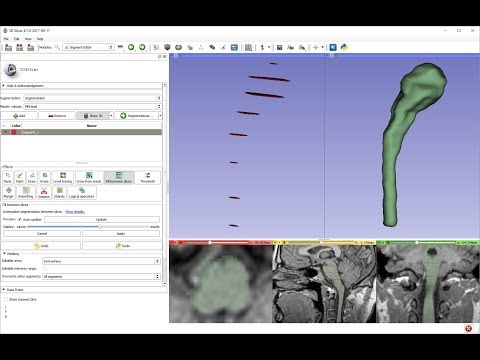
Notes:

• Only visible segments are used by this effect.
• The method does not use the master volume, only the shape of the specified segments.
• The method uses ND morphological contour interpolation algorithm. See details here: http://insight-journal.org/browse/publication/977

Threshold

Use Threshold to determine a threshold range and save results to selected segment or use it as Editable intensity range.

Margin

Grows or shrinks the selected segment by the specified margin.

Smoothing

Smoothes selected labelmap or all labelmaps (only for Joint smoothing method).

By clicking Apply button, the entire segmentation is smoothed.

To smooth a specific region, left click and drag in any slice or 3D view. Same smoothing method and strength is used as for the whole-segmentation mode (size of the brush does not affect smoothing strength, just makes it easier to designate a larger region).

Available methods:

• Median: removes small extrusions and fills small gaps while keeps smooth contours mostly unchanged. Applied to selected segment only.
• Opening: removes extrusions smaller than the specified kernel size. Does not add anything to the segment. Applied to selected segment only.
• Closing: fills sharp corners and holes smaller than the specified kernel size. Does not remove anything from the segment. Applied to selected segment only.
• Gaussian: smoothes all details. Strong smoothing as achievable, but tends to shrink the segment. Applied to selected segment only.
• Joint smoothing: smoothes multiple segments at once, preserving watertight interface between them. If segments overlap, segment higher in the segments table will have priority. Applied to all visible segments.

Scissors

Clip segments to the specified region or fill regions of a segment (typically used with masking). Regions can be drawn on both slice view or 3D views.

• Left click to start drawing (free-form or rubber band circle or rectangle)
• Release button to apply

Islands

Use this tool to create a unique segment for each connected region of the selected segment. Connected regions are defined as groups of pixels which touch each other but are surrounded by zero valued voxels.

• Fully connected: If checked then only voxels that share a face are counted as connected; if unchecked then voxels that touch at an edge or a corner are considered connected.
• Minimum size: All regions that have less than this number of voxels will be deleted.

Logical operators

Apply Boolean operators to selected segment or combine segments.

Mask volume

Blank out inside/outside of a segment in a volume or create a binary mask. Result can be saved into a new volume or overwrite the input volume. This is useful for removing irrelevant details from an image (for example remove patient table; or crop the volume to arbitrary shape for volume rendering) or create masks for image processing operations (such as registration or intensity correction).

• Fill inside: set all voxels of the selected volume to the specified value inside the selected segment
• Fill outside: set all voxels of the selected volume to the specified value outside the selected segment
• Fill inside and outside: create a binary labelmap volume as output. Most image procesing operations require background (outside, ignored) region to be filled with 0 value.

Tips

• A large radius paint brush with threshold painting is often a very fast way to segment anatomy that is consistently brighter or darker than the surrounding region, but partially connected to similar nearby structures (this happens a lot).
• Use the slice viewer menus to control the label map opacity and display mode (to show outlines only or full volume).

Frequently asked questions

Cannot paint outside some boundaries

When you create a segmentation, internal labelmap geometry (extent, origin, spacing, axis directions) is determined from the master volume that you choose first. You cannot paint outside this extent.

If you want to extend the segmentation to a larger region then you need to modify segmentation’s geometry using “Specify geometry” button.

Segmentation is not accurate enough

If details cannot be accurately depicted during segmentation or the exported surface has non-negligible errors (there are gaps or overlap between segments), then it is necessary to reduce the segmentation’s spacing (more accurately: spacing of the internal binary labelmap representation in the segmentation node). Spacing is also known as voxel size or may be referred to as resoution (which is inverse of spacing - higher resolution means smaller spacing).

As a general rule, segmentation’s spacing needs to be 2-5x smaller than the size of the smallest relevant detail or the maximum acceptable surface error in the generated surface.

By default, segmentation’s spacing is set from the master volume that is selected first after the segmentation is created. If the first selected master volume’s resolution is not sufficient or highly anisotropic (spacing value is not the same along the 3 axes) then one of the followings is recommended:

• Option A. Crop and resample the input volume using Crop volume module before starting segmentation. Make spacing smaller (small enough to represent all details but not too small to slow things down and consume too much memory) and isotropic by reducing Spacing scale and enabling Isotropic spacing. Also adjust the region of interest to crop the volume to minimum necessary size to minimize memory usage and make editing faster.
• Option B. Click Specify geometry button in Segment Editor any time to specify smaller spacing. After this smooth segments using Smoothing effect. Joint smoothing method is recommended as it can smooth all the segments at once and it preserves boundaries between segments. Joint smoothing flattens all the processed segments into one layer, so if the segentation contains overlapping segments then segment in several steps, in each step only show a set of non-overlapping segments (or use any of the other smoothing methods, which only operate on the selected segment).

Generated surface contains step artifacts

If 3D surface generated from the segmentation contains step artifacts (looks “blocky”) then it is necessary to increase smoothing and/or reduce segmentation’s spacing.

Users need to choose between having smooth surface vs. no gaps or overlap between segments. It is impossible to have both. To achieve the desired results, there are two parameters to control: segmentation’s spacing and surface smoothing factor:

1. Choose spacing that allows accurate segmentation (see Segmentation is not accurate enough section above)
2. Choose smoothing value that removes staircase artifacts but still preserves all details that you are interested in.
3. If you find that the surface smoothing value that is high enough to remove staircase artifacts also removes relevant details then further reduce spacing.

Paint affects neighbor slices or stripes appear in painted segments

Segment Editor allows editing of segmentation on slices of arbitrary orientation. However, since edited segments are stored as binary labelmaps, “striping” artifacts may appear on thin segments or near boundary of any segments. See Oblique segmentation segmentation recipe for more details and instructions on how to deal with these artifacts.

Limitations

• Threshold will not work with non-scalar volume background volumes.
• Mouse wheel can be used to move slice through volume, but on some platforms (mac) it may move more than one slice at a time.

Related Modules

• Segment Statistics module computes volume, surface, mean intensity, and various other metrics for each segment.
• Segmentations module allows changing visualization options, exporting/importing segments to/from other nodes (models, labelmap volumes), and moving or copying segments between segmentation nodes.
• Data module shows all segmentations and segments in a tree structure. Commonly used operations are available by right-clicking on an item in the tree.
• Editor module is the predecessor of this module. Segment Editor provides all its features and many more.

Information for Developers

See examples for creating and modifying segmentation nodes and using segment editor effects from your own modules in Slicer script repository

Contributors

Authors:

• Csaba Pinter (PerkLab, Queen’s University)
• Andras Lasso (PerkLab, Queen’s University)
• Kyle Sunderland (PerkLab, Queen’s University)
• Steve Pieper (Isomics Inc.)
• Wendy Plesniak (SPL, BWH)
• Ron Kikinis (SPL, BWH)
• Jim Miller (GE)

Acknowledgements

This module is partly funded by an Applied Cancer Research Unit of Cancer Care Ontario with funds provided by the Ministry of Health and Long-Term Care and the Ontario Consortium for Adaptive Interventions in Radiation Oncology (OCAIRO) to provide free, open-source toolset for radiotherapy and related image-guided interventions. The work is part of the National Alliance for Medical Image Computing <http://www.na-mic.org/>_ (NA-MIC), funded by the National Institutes of Health through the NIH Roadmap for Medical Research, Grant U54 EB005149.

Segment statistics

This is a module for the calculation of statistics related to the structure of segmentations, such as volume, surface area, mean intensity, and various other metrics for each segment.

Labelmap statistics

Labelmap statistics are calculated using the binary labelmap representation of the segment.

• Voxel count: the number of voxels in the segment
• Volume mm3 the volume of the segment in mm3
• Volume cm3 the volume of the segment in cm3
• Centroid: the center of mass of the segment in RAS coordinates
• Feret diameter: the diameter of a sphere that can encompass the entire segment
• Surface area mm2: the volume of the segment in mm2
• Roundness: the roundness of the segment. Calculated from ratio of the area of the sphere calculated from the Feret diameter by the actual area. Value of 1 represents a spherical structure. See detailed definition here.
• Flatness: the flatness of the segment. Calculated from square root of the ratio of the second smallest principal moment by the smallest. Value of 0 represents a flat structure. See detailed definition here.
• Elongation: the elongation of the segment. Calculated from square root of the ratio of the second largest principal moment by the second smallest. See detailed definition here.
• Principal moments: the principal moments of inertia for each axes of the segment
• Principal axes: the principal axes of rotation of the segment
• Oriented bounding box: the non-axis aligned bounding box that encompasses the segment

Scalar volume statistics

• Voxel count: the number of voxels in the segment
• Volume mm3 the volume of the segment in mm3
• Volume cm3 the volume of the segment in cm3
• Minimum: the minimum scalar value behind the segment
• Maximum: the maximum scalar value behind the segment
• Mean: the mean scalar value behind the segment
• Median: the median scalar value behind the segment
• Standard deviation: the standard deviation of scalar values behind the segment

Closed surface statistics

• Surface area mm2: the volume of the segment in mm2
• Volume mm3 the volume of the segment in mm3
• Volume cm3 the volume of the segment in cm3

Related Modules

• Segmentations module allows changing visualization options, exporting/importing segments to/from other nodes (models, labelmap volumes), and moving or copying segments between segmentation nodes.
• Segment Editor module for segmentation of volumes using tools for editing (paint, draw, erase, level tracing, grow from seeds, threshold, etc.)

Information for developers

See examples for calculating statistics from your own modules in the Slicer script repository <https://www.slicer.org/wiki/Documentation/Nightly/ScriptRepository#Quantifying_segments>. Additional plugins for computation of other statistical measurements may be registered by subclassing SegmentStatisticsPluginBase.py <https://github.com/Slicer/Slicer/blob/master/Modules/Scripted/SegmentStatistics/SegmentStatisticsPlugins/SegmentStatisticsPluginBase.py>, and registering the plugin with SegmentStatisticsLogic.

Contributors

Authors:

• Csaba Pinter (PerkLab, Queen’s University)
• Andras Lasso (PerkLab, Queen’s University)
• Christian Bauer (University of Iowa)
• Steve Pieper (Isomics Inc.)
• Kyle Sunderland (PerkLab, Queen’s University)

Acknowledgements

This module is partly funded by an Applied Cancer Research Unit of Cancer Care Ontario with funds provided by the Ministry of Health and Long-Term Care and the Ontario Consortium for Adaptive Interventions in Radiation Oncology (OCAIRO) to provide free, open-source toolset for radiotherapy and related image-guided interventions. The work is part of the National Alliance for Medical Image Computing <http://www.na-mic.org/>_ (NA-MIC), funded by the National Institutes of Health through the NIH Roadmap for Medical Research, Grant U54 EB005149.

Transforms

Overview

This module is used for creating, editing, and visualization of spatial transformations. Transformations are stored in transform nodes and define position, orientation, and warping in the world coordinate system or relative to other nodes, such as volumes, models, markups, or other transform nodes.

See a summary of main features demonstrated in this video.

Supported transform types:

• linear transform: rigid, scaling, shearing, affine, etc. specified by a 4x4 homogeneous transformation matrix
• b-spline transform: displacement field specified at regular grid points, with b-spline interpolation
• grid transform: dense displacement field, with trilinear interpolation
• thin-plate splines: displacements specified at arbitrarily placed points, with thin-plate spline interpolation
• composite transforms: any combinations of the transforms above, in any order, any of them optionally inverted

Use cases

Create a transform

Transform node can be created in multiple ways:

• Method A: In Data module’s Subject hierarchy tab, right-click on the “Transform” column and choose “Create new transform”. This always creates a general “Transform”.
• Method B: In Data module’s Transform hierarchy tab, right-click on an item and choose “Insert transform”. This always creates a “Linear transform”. Advantage of this method is that it is easy to build and overview hierarchy of transforms.
• Method C: In Transforms module click on “Active transform” node selector and choose one of the “Create new…” options.

How to choose transform type: Create “Linear transform” if you only work with linear transforms, because certain modules only allow you to select this node type as input. In other cases, it is recommended to create the general “Transform” node. Multiple transform node types exist because earlier Slicer could only store a simple transformation in a node. Now a transform node can contain any transformation type (linear, grid, bspline, thin-plate spline, or even composite transformation - an arbitrary sequence of any transformations), therefore transform node types only differ in their name. In some modules, node selectors only accept a certain transform node type, therefore it may be necessary to create that expected transform type, but in the long term it is expected that all modules will accept the general “Transform” node type.

Apply transform to a node

“Applying a transform” means setting parent transform to a node to translate, rotate, and/or warp it. If the parent transform is changed then the position or shape of the node is automatically updated. If the transform is removed then original (non-transformed) state of the node is restored.

A transform can be applied to a node in multiple ways:

• Method A: In Data module’s Subject hierarchy tab, right-click on the “Transform” column and choose a transform (or “Create new transform”). The transform can be interactively edited in 3D views by right-click on “Transform” column and choosing “Interaction in 3D view”. See this short demonstration video.
• Method B: In Data module’s Transform hierarchy tab, drag the nodes under a transform.
• Method C: In Transforms module’s “Apply transform” section move nodes from the Transformable list to the Transformed list by selecting them and click the arrow button between them.

Parent transform can be set for transform nodes, thereby creating a hierarchy (tree) of transforms. This transform tree is displayed in Data module’s Transform hierarchy tab.

Harden transform on a node

“Hardening a transform” means permanently modify the node according to the currently applied transform. For example, coordinate values of model points are updated with the transformed coordinates, or a warped image voxels are resampled. After hardening the transform, the node is no longer associated with the transform.

A transform can be hardened on a node in multiple ways:

• Method A: In Data module, right-click on Transform column and click “Harden transform”
• Method B: In Transforms module’s “Apply transform” section, click the harden button (below the left arrow button).

If non-linear transform is hardened on a volume then the volume is resampled using the same spacing and axis directions as the original volume (using linear interpolation). Extents are updated to fully contain the transformed volume. To specify a different image extent or resolution, one of the image resampling modules can be used, such as “Resample Scalar/Vector/DWI volume”.

Modify transform

• Invert: all transforms can be inverted by clicking “Invert” button in Transforms module’s Edit section. This is a reversible operation, as the transform’s internal representation is not changed, just a flag is set that the transform has to be interpreted as its inverse.
• Split: a composite transform can be split to multiple transform nodes (so that each component is stored in a separate transform node) by clicking “Split” button in Transforms module’s Edit section.
• Change translation/rotation:
  • linear transforms can be edited using translation and rotation sliders Transforms module’s Edit section. “Translation in global or local reference frame” button controls if translation is performed in the parent coordinate system or the rotated coordinate system.
  • translation and rotation of a linear transform can be interactively edited in 3D by enabling “Visible in 3D view” in Transform’s module Display / Interaction section. See this short demonstration video.
• Edit warping transform: to specify/edit a warping transform that translates a set of points to specified positions, you can use semi-automatic registration methods

Compute transform

Transforms are usually computed using spatial registration tools.

Save transform

Traansforms are saved into ITK transform file format. ITK always saves transform “from parent”, as this is the direction that is necessary for transforming images.

If a transform node in Slicer has a transformation with “to parent” direction (e.g., it was computed like that or a “from parent” transform got inverted) then:

• linear transforms: the transform is automatically converted to “from parent” direction. See [developer page](See examples and other developer information in Developer guide for more details about this conversion.
• warping transforms: the transform is saved as special inverse transform class that most ITK-based applications cannot interpret. If compatibility with other applications is needed, the transform can be converted to a displacement field before saving.

A quick way to export a linear transform to another software or to text files is to copy the homogeneous transformation matrix values to the clipboard by clicking “Copy” button in Edit section in Transforms module.

Load transform

Drag-and-drop the transform file to the application window and make sure “Transform” is selected in Description column.

MetaImage (mha), NIFTI (nii) vector volumes can be loaded as displacement field (grid) transform. The volume and its vectors are expected to be stored in LPS coordinate system (during reading they are converted to RAS to match coordinate system conventions in Slicer).

A quick way to import a linear transform from another software or from text files is to copy the homogeneous transformation matrix values to the clipboard, and click “Paste” button in Edit section in Transforms module.

Visualize transform

Transforms can be visualized in both 2D and 3D views, as glyphs representing the displacement vectors as arrows, cones, or spheres; regular grids that are deformed by the transform; or contours that represent lines or surfaces where the displacement magnitude has a specific value. See documentation of [Display section](transforms.html#display] for details.

Panels and their use

Active Transform: Select the transform node to display, control and edit.

Information

Displays details about what transformation(s) a transform node contains, such as type and direction (”to parent” or “from parent).

It also displays displacement value at the current mouse pointer position (in slice views, it is enough to just move the mouse pointer; in 3D views, Shift key must be held down while moving the mouse).

Edit

• Transform matrix: 4x4 homogeneous transformation matrix. Each element is editable on double click. Type Enter to validate change, Escape to cancel or Tab to edit the next element. First 3 columns of the matrix specifies an axis of the transformed coordinate system. Scale factor along an axis is the column norm of the corresponding column. Last column specifies origin of the transformed coordinate system. Last row of the transform is always [0, 0, 0, 1].
• Translation and rotation sliders:
  • Translation: Apply LR, PA, and IS translational components of the transformation matrix in RAS space (in mm). Min and Max control the lower and upper bounds of the sliders.
  • Rotation: Apply LR, PA, and IS rotation angles (degrees) in the RAS space. Rotations are concatenated.
  • Note: Linear transform edit sliders only show relative translation and rotation because a transformation can be achieved using many different series of transforms. To make this clear to users, only one transform slider can be non-zero at a time (all previously modified sliders are reset to 0 when a slider is moved). The only exception is translation sliders in “translate first” mode (i.e., when translation in global/local coordinate system button is not depressed): in this case there is a only one way how a specific translation can be achieved, therefore transform sliders are not reset to 0. An rotating dial widget would be a more appropriate visual representation of the behavior than sliders, but slider is chosen because it is a standard widget and users are already familiar with it.
• Translation reference frame: Determines what coordinate system the translation (specified by translation sliders) is specified in - in the parent coordinate system or in the rotated coordinate system.
• Identity: Resets transformation matrix to identity matrix.
• Invert: Inverts the transformation matrix.
• Split: Split a composite transform so that each of its component is stored in a separate transform node.
• Copy: copy the homogeneous transformation matrix values to the clipboard. Values are separated by spaces, each line of the transform is in a separate line.
• Paste: paste transformation matrix from clipboard. Values can be separated by spaces, commas, or semicolons, which allows copy/pasting numpy array from Python console or matrix from Matlab.

Display

This section allows visualization of how much and what direction of displacements specified by the transform.

Visualization modes

1. Glyph mode

Slice view:

• arrow: the arrow shows the displacement vector at the arrow starting point, projected to the slice plane
• cone: the cone shows the displacement vector at the cone centerpoint, projected to the slice plane
• sphere: the circle diameter shows the displacement vector magnitude at the circle centerpoint

Glyph - arrow (slice view)	Glyph - cone (slice view)	Glyph - sphere (slice view)

3D view:

• arrow: the arrow shows the displacement vector at the arrow starting point
• cone: the cone shows the displacement vector at the cone centerpoint
• sphere: the sphere diameter shows the displacement vector magnitude at the circle centerpoint

Glyph - arrow (3D view)	Glyph - cone (3D view)	Glyph - sphere (3D view)

1. Grid mode

• Slice view: Grid visualization (2D): shows a regular grid, deformed by the displacement vector projected to the slice
• 3D view: shows a regular grid, deformed by the displacement vector

Grid (slice view)	Grid - slice plane (3D view)	Grid - volume (3D view)

1. Contour mode

• Slice view: iso-lines corresponding to selected displacement magnitude values
• 3D view: iso-surfaces corresponding to selected displacement magnitude values

Contour (slice view)	Contour (3D view)

Coloring

Open Transforms module / Display section / Colors section. If you click on a small circle then above the color bar you can see the small color swatch. On its left side is the points index (an integer that tells which point is being edited and that can be used to jump to the previous/next point), and on its right side is the mm value corresponding to that color.

The default colormap is:

• 1mm (or below) = gray
• 2mm = green
• 5mm = yellow
• 10mm (or above) = red

You can drag-and-drop any of the small circles or modify the mm value in the editbox. You can also add more color values by clicking on the color bar. Then, you can assign a color and/or adjust the mm value. If you click on a circle and press the DEL key then the color value is deleted.

If you need to know accurate displacement values at specific positions then switch to contour mode and in the “Levels” list enter all the mm values that you are interested in. For example, if you enter only a single value “3” in the Levels field you will see a curve going through the points where the displacement is exactly 3 mm; on one side of the curve the displacements are smaller, on the other side the displacements are larger.

You can show both contours and grid or glyph representations by loading the same transform twice and choosing a different representation for each.

Apply transform

Controls what nodes the currently selected “Active transform” is applied to.

• Transformable: List the nodes in the scene that do not directly use the active transform node.
• Transformed: List the nodes in the scene that use the active transform node.
• Right arrow: Apply the active transform node to the selected nodes in Transformable list.
• Left arrow: Remove the active transform node from the selected nodes in the Transformed list.
• Harden transform: Harden active transform on the nodes selected in the Transformed list.

Convert

This section can sample the active transform on a grid (specified by the selected “Reference volume”) and save it to a node. Depending on the type of selected “Output displacement field” node, slightly different information is exported:

• Scalar volume node : magnitude of displacement is saved as a scalar volume
• Vector volume node: displacement vectors are saved as voxel values (in RAS coordinate system). When the vector volume is written to file, the image grid is saved in LPS coordinate system, but displacement values are still kept in RAS coordinate system.
• Transform node: a grid transform is constructed. This can be used for creating an inverted displacement field that any ITK application can read. When the grid transform is written to file, both the image grid and displacement values are saved in LPS coordinate system.

Related modules

• Registration modules: transforms can be computed automatically using semi-automatic or automatic registration modules

Information for developers

See examples and other developer information in Developer guide and Script repository.

Contributors

• Alex Yarmarkovich (Isomics, SPL)
• Jean-Christophe Fillion-Robin (Kitware)
• Julien Finet (Kitware)
• Andras Lasso (PerkLab, Queen’s)
• Franklin King (PerkLab, Queen’s)

Acknowledgements

This work is funded in part by the National Institutes of Health through the NIH Roadmap for Medical Research, Grant U54 EB005149.

Volume rendering

Overview

Volume rendering (also known as volume ray casting) is a visualization technique for displaying image volumes as 3D objects directly - without requiring segmentation.

This is accomplished by specifying color and opacity for each voxel, based on its image intensity. Several presets are available for this mapping, for displaying bones,soft tissues, air, fat, etc. on CT and MR images. Users can fine-tune these presets for each image.

Use cases

Display a CT or MRI volume

• Load a data set (for example, use Sample Data module to load “CTChest” data set)
• Go to Data module
• Show volume rendering:
  • Option A: drag-and-drop the volume in the subject hierarchy tree into a 3D view
  • Option B: right-click on the eye icon, and choose “Show in 3D views as volume rendering”

To adjust volume rendering settings

• Right-click on the eye icon and choose “Volume rendering options” to switch to edit visualization options in Volume rendering module
• Choose a different preset in Display section,
• Adjust “Offset” slider to change what image intensity range is visible

Render different volumes in two views

Switch to a layout with multiple 3D views (for example “Dual 3D”) using the toolbar and then use one of the two options below.

Option A:

• Go to Data module and drag-and-drop each volume into the 3D view

Option B:

• Go to Volume Rendering module
• Open the “Inputs” section
• Select the first volume
• Click View list and uncheck “View2” (only “View1” should be checked)
• Click the eye icon for the volume to show up in “View1”
• Select the second volume
• Click View list and uncheck “View1” (only “View2” should be checked)
• Click the eye icon for the volume to show up in “View2”

Limitations

• Only single-component scalar volumes can be used for volume rendering. Vector to Scalar Volume module can convert vector volume to scalar volume.
• To render multiple overlapping volumes, select “VTK Multi-Volume” rendering in “Display” section. Currently, no cropping can be applied in this mode.
• To reduce staircase artifacts during rendering, choose enable “Surface smoothing” in Advanced/Techniques/Advanced rendering properties section, or choose “Normal” or “Maximum” as quality.

Panels and their use

• Inputs: Contains the list of nodes required for VolumeRendering. It is unlikely that you need to interact with controllers.
  • Volume: Select the current volume to render. Note that only one volume can be rendered at a time.
  • Display: Select the current volume rendering display properties. Volume rendering display nodes contains all the information relative to volume rendering. They contain pointers to the ROI, volume property and view nodes. A new display node is automatically created if none exist for the current volume.
  • ROI: Select the current ROI to optionally crop with 6 planes the volume rendering.
  • Property: Select the current Volume Property. Volume properties contain the opacity, color and gradient transfer functions for each component.
  • View: Select the 3D views where the volume rendering must be displayed into. If no view is selected, the volume rendering is visible in all views
• Display: Main properties for the volume rendering.
  • Preset: Apply a pre-defined set of functions for the opacity, color and gradient transfer functions. The generic presets have been tuned for a combination of modalities and organs. They may need some manual tuning to fit your data.
  • Shift: Move all the inner points (first and last excluded) of the current transfer functions to the right/left (lower/higher). It can be useful when a preset defines a ramp from 0 to 200 but your data requires a ramp from 1000 to 1200.
  • Crop: Simple controls for the cropping box (ROI). More controls are available in the “Advanced…” section. Enable/Disable cropping of the volume. Show/Hide the cropping box. Reset the box ROI to the volume’s bounds.
  • Rendering: Select a volume rendering method. A default method can be set in the application settings Volume Rendering panel.
    • VTK CPU Ray Casting: Available on all computers, regardless of capabilities of graphics hardware. The volume rendering is enterily realized on the CPU, therefore it is slower than other options.
    • VTK GPU Ray Casting (default): Uses graphics hardware for rendering, typically much faster than CPU volume rendering. This is the recommended method for computers that have sufficiant graphics capabilities. It supports surface smoothing to remove staircase artifacts.
    • VTK Multi-Volume: Uses graphics hardware for rendering. Can render multiple overlapping volumes. Currently does not support cropping.
• Advanced: More controls to control the volume rendering. Contains 3 tabs: “Techniques”, “Volume Properties” and “ROI”
  • Techniques: Advanced properties of the current volume rendering method.
    • Quality:
      • Adaptive: quality is reduced while interacting with the view (rotating, changing volume rendering settings, etc.).
        • Interactive speed: Ensure the given frame per second (FPS) is enforced in the views during interaction. The higher the FPS, the lower the resolution of the volume rendering
      • Normal (default): fixed rendering quality, should work well for volumes that the renderer can handle without difficulties.
      • Maximum: oversamples the image to achieve higher image quality, at the cost of slowing down the rendering.
    • Auto-release resources: When a volume is shown using volume rendering then graphics resources are allocated (GPU memory, precomputed gradient and space leaping volumes, etc.). This flag controls if these resources are automatically released when the volume is hidden. Releasing the resources reduces memory usage, but it increases the time required to show the volume again. Default value can be set in application settings Volume Rendering panel.
    • Technique:
      • Composite with shading (default): display as a shaded surface
      • Maximum intensity projection: display brightest voxel value encountered in each projection line
      • Minimum intensity projection: display darkest voxel value encountered in each projection line
    • Surface smoothing: check this checkbox to reduce staircase artifacts by adding a random noise pattern (jitter) to the raycasting lines
  • Volume Properties: Advanced views of the transfer functions.
    • Synchronize with Volumes module: show volume rendering with the same color mapping that is used in slice views
      • Click: Apply once the properties (window/level, threshold, lut) of the Volumes module to the Volume Rendering module.
      • Checkbox: By clicking on the checkbox, you can toggle the button. When toggled, any modification occuring in the Volumes module is continuously applied to the volume rendering
    • Control point properties: X = scalar value, O = opacity, M = mid-point, S = sharpness
    • Keyboard/mouse shortcuts:
      • Left button click: Set current point or create a new point if no point is under the mouse.
      • Left button move: Move the current or selected points if any.
      • Right button click: Select/unselect point. Selected points can be moved at once
      • Right button move: Define an area to select points:
      • Middle button click : Delete point under the mouse cursor.
      • Right/Left arrow keys: Change of current point
      • Delete key: Delete the current point and set the next point as current
      • Backspace key : Delete the current point and set the previous point as current
      • ESC key: Unselect all points.
    • Scalar Opacity Mapping: Opacity transfer function. Threshold mode: enabling threshold controls the transfer function using range sliders in addition to control points.
    • Scalar Color Mapping: Color transfer function.
    • Gradient Opacity: Gradient opacity transfer function. This controls the opacity according to how large a density gradient next to the voxel is.
    • Advanced:
      • Interpolation: Linear (default for scalar volumes) or nearest neighboor (default for labelmaps) interpolation.
      • Shade: Enable/Disable shading. Shading uses light and material properties. Disable it to display X-ray-like projection.
      • Material: Material properties of the volume to compute shading effect.
  • ROI: More controls for the cropping box.
    • Display Clipping box: Show hide the bounds of the ROI box.
    • Interactive mode: Control wether the cropping box is instantaneously updated when dragging the sliders or only when the mouse button is released.

Contributors

• Julien Finet (Kitware)
• Alex Yarmarkovich (Isomics)
• Csaba Pinter (PerkLab, Queen’s University)
• Andras Lasso (PerkLab, Queen’s University)
• Yanling Liu (SAIC-Frederick, NCI-Frederick)
• Andreas Freudling (SPL, BWH)
• Ron Kikinis (SPL, BWH)

Acknowledgements

This work is part of the National Alliance for Medical Image Computing (NAMIC), funded by the National Institutes of Health through the NIH Roadmap for Medical Research, Grant U54 EB005149. Some of the transfer functions were contributed by Kitware Inc. (VolView)

Volumes

Overview

Volumes module provides basic information about volume nodes, can convert between volume types, and allows adjustment of display settings.

A volume node stores 3D array of elements (voxels) in a rectilinear grid. Grid axes are orthogonal to each other and can be arbitrarily positioned and oriented in physical space. Grid spacing (size of voxel) may be different along each axis.

Volume nodes have subtypes, based on what is stored in a voxel:

• Scalar volume: most common type of volume, voxels represent continuous quantity, such as a CT or MRI volume.
• Labelmap volume: each voxel can store a discrete value, such as an index or label; most commonly used for storing a segmentation, each label corresponds to a segment.
• Vector volume: each voxel stores multiple scalar values, such as RGB components of a color image, or RAS components of a displacement field.
• Tensor volume: each voxel stores a tensor, typically used for storing MRI diffusion tensor image.

Scalar volume	Labelmap volume	Vector volume	Tensor volume

Volumes module handles a 2D image as a single-slice 3D image. 4D volumes are represented as a sequence of 3D volumes, using Sequences extension.

Use cases

Display volume

Slice views: After loading a volume, it is displayed in slice views by default. If multiple volumes are loaded, Data module can be used to choose which one is displayed. Slice view controls allow further customization of which volume is displayed in which view and how.

3D views: Volumes can be displayed in 3D views using Volume rendering module. If structures of interest cannot be distinguished from surrounding regions then it may be necessary to segment the image using Segment Editor module and click Show 3D button.

Overlay two volumes

• Load two volumes
• Go to Data module
• Left-click on the “eye” icon of one of the volumes to show it as background volume
• Right-click on “eye” icon of the other volume and choose “Show in slice views as foreground”
• Adjust transparency of the foreground volume using the vertical slider in slice view controls. Click link button to make all changes applied to all slice views (in the same view group)

Load image file as labelmap volume

By default, a single-component image is loaded as scalar volume. To make Slicer interpret an image as labelmap volume, either of these options can be used:

• A. When the file is selected for loading, in Add data... dialog, check Show Options to see additional options, and check LabelMap checkbox in Volumes module.
• B. Before loading the file, rename it so that it contains label or seg in its name, for example: something.label.nrrd, something-label.nrrd, or something-seg.nrrd. This makes LabelMap checked by default.
• C. Load the file as scalar volume, and then convert it to labelmap volume by clicking Convert button at the bottom of Volume information section

If the goal is to load an image as labelmap volume so that it can be converted to segmentation, then simpler options available:

• A. Choose Segmentation in Description column in Add data... window. This only works for nrrd and nifti images.
• B. Sve the volume in nrrd file format and rename it to have .seg.nrrd extension, for example: something.seg.nrrd. This makes the file loaded as Segmentation by default.

Load a series of png, jpeg, or tiff images as volume

Consider the Image Stacks provided by the SlicerMorph extension to work with large sets of high resolution images. It allows you to automatically convert RGB to grayscale scalar volume, specify image spacing, and downsample large images.

Alternatively you can load and manipulate the data directly using functionality in the core Slicer modules:

• Choose from the menu: File / Add Data
• Click Choose File(s) to Add button and select any of the files in the sequence in the displayed dialog. Important: do not choose multiple files or the entire parent folder, just a single file of the sequence. All file names must start with a common prefix followed by a frame number (img001.tif, img002.tif,…). Number of rows and columns of the image must be the same in all files.
• Check Show Options and uncheck Single File option
• Click OK to load the volume
• Go to the Volumes module
• Choose the loaded image as Active Volume
• In the Volume Information section set the correct Image Spacing and Image Origin values
• Most modules require grayscale image as input. The loaded color image can be converted to a grayscale image by using the Vector to scalar volume module

These steps are also demonstrated in this video.

Note: Consumer file formats, such as jpg, png, and tiff are not well suited for 3D medical image storage due to the following serious limitations:

• Storage is often limited to bit depth of 8 bits per channel: this causes significant data loss, especially for CT images.
• No standard way of storing essential metadata: slice spacing, image position, orientation, etc. must be guessed by the user and provided to the software that imports the images. If the information is not entered correctly then the images may appear distorted and measurements on the images may provide incorrect results.
• No standard way of indicating slice order: data may be easily get corrupted due to incorrectly ordered or missing frames.

Panels and their use

• Active Volume: Select the volume to display and operate on.
• Volume Information: Information about the selected volume. Some fields can be edited to correctly describe the volume, for example, when loading incompletely specified image data such as a sequence of jpeg files. Use caution however, since changing properties such as Image Spacing will impact the physical accuracy of some calculations such as Label Statistics.
  • Image Dimensions: The number of pixels in “IJK” space - this is the way the data is arranged in memory. The IJK indices (displayed in the DataProbe) go from 0 to dimension-1 in each direction.
  • Image Spacing: The physical distance between pixel centers when mapped to patient space expressed in millimeters.
  • Image Origin: The location of the center of the 0,0,0 (IJK) pixel expressed with respect to patient space. Patient space is organized with respect to the subject’s Right, Anterior, and Superior anatomical directions. See coordinate systems page for more information.
  • IJK to RAS Direction Matrix: The trasnform matrix from the IJK to RAS coordinate systems
  • Center Volume: This button will apply a transform to the volume that shifts its center to the origin in patient space. Harden the transform on the volume to permanently change the image origin.
  • Scan Order: Describes the image orientation (how the IJK space is oriented with respect to patient RAS.
  • Number of Scalars: Most CT or MR scans have one scalar component (grayscale). Color images have three components (red, green, blue). Tensor images have 9 components.For diffusion weighted volumes this indicates the number of baseline and gradient volumes.
  • Scalars Type: Tells the computer representation of each voxel. Volume module works with all types, but most modules expect scalar volumes. Vector volumes can be converted to scalar volumes using Vector to Scalar Volume module.
  • Filename: Path to the file which this volume was loaded from/saved to
  • Window/Level Presets: Loaded from DICOM headers defined by scanner or by technician.
  • Convert to label map / Convert to scalar volume: Convert the active volume between labelmap and scalar volume.
• Display: Set of visualization controls appropriate for the currently selected volume. Not all controls are available for all volume types.
  • Lookup Table: Select the color mapping for scalar volumes to colors.
  • Interpolate: When checked, slice views will display linearly interpolated slices through input volumes. Unchecked indicates nearest neighbor resampling
  • Window Level Presets: Predefinied shortcuts to window/level and color table combinations for common visualization requirements.
  • Window/Level Controls: Double slider with text input to define the range of input volume data that should be mapped to the display grayscale. Auto window level tries to estimate the intensity range of the foreground image data. On mouse over, a popup slides down to add support for large dynamic range by giving control over the range of the window level double slider.
  • Threshold: Controls the range of the image that should be considered transparent when used in the foreground layer of the slice display. Same parameters also control transparency of slice models displayed in the 3D viewers.
  • Histogram: Shows the number of pixels (y axis) vs the image intensity (x axis) over a background of the current window/level and threshold mapping.
• Diffusion Weighted Volumes: The following controls show up when a DWI volume is selected
  • DWI Component: Selects the baseline or diffusion gradient direction volume to display.
• Diffusion Tensor Volumes: The following controls show up when a DTI volume is selected
  • Scalar Mode: Mapping from tensor to scalar.
  • Slice Visibility: Allows display of graphics visualizations of tensors on one or more of the standard Red, Green, or Yellow slice views.
  • Opacity: How much of the underlying image shows through the glyphs.
  • Scalar Color Map: How scalar measures of tensor are mapped to color.
  • Color by Scalar: Which scalar metric is used to determine the color of the glyphs.
  • Scalar Range: Defines the min-max range of the scalar mapping to color. When enabled, allows a consistent color mapping independent of the full range of the currently displayed item (if not selected color range will cover min-max of the currently displayed data).
  • Glyph Type: Tubes and line show direction of eigen vector of tensor (major, middle, or minimum as selected by the Glyph Eigenvector parameter). Ellipsoid shows direction and relative scale of all three eigenvectors.
  • Scale Factor: Controls size of glyphs. There are no physical units for this parameter.
  • Spacing: Controls the number of glyphs on the slice view.

Related modules

• Volume rendering: visualize volume in 3D views without segmentation
• Segment editor: delineate structures in the volume for analysis and 3D visualization
• Vector to scalar volume: convert vector volume to scalar volume
• Extensions:
  • Image Maker: create a volume from scratch
  • Image Stacks provided by the SlicerMorph extension.

Contributors

• Steve Piper (Isomics)
• Julien Finet (Kitware)
• Alex Yarmarkovich (Isomics)
• Nicole Aucoin (SPL, BWH)

Acknowledgements

This work is part of the National Alliance for Medical Image Computing (NAMIC), funded by the National Institutes of Health through the NIH Roadmap for Medical Research, Grant U54 EB005149.

Extensions Manager

Application settings

Editing application settings

The application settings dialog allows users to customize application behavior.

After starting Slicer, it can be accessed clicking in menu: Edit / Application Settings.

General

Application startup script can be used to launch any custom Python code when Slicer application is started.

Modules

Skip loading

Select which type of modules to not load at startup. It is also possible to start slicer by temporarily disabling those modules (not saved in settings) by passing the arguments in the command line.

For example, this command will start Slicer without any CLI loaded:

Slicer.exe --disable-cli-modules

Prefer Executable CLIs

Use the executable version of a CLI instead of its shared version. CLI modules typically come in 2 forms, as shared (dll)and as executable (exe). By default, if there is a shared version, it is the one loaded by Slicer, ignoring the executable version. Loading a shared runs the module faster but increases the memory consumption. For some configurations (e.g. Windows 32b), memory is critical. Toggling this option to ON skips the loading of shared CLIs and loads executable version of CLIs instead. If there is no executable for a given CLI, the shared version is used.

Show hidden modules

Some modules don’t have a user interface, they are hidden from the module’s list. For debugging purpose, it is possible to force their display

Temporary directory

Directory where modules can store their temporary outputs if needed.

Additional module paths

List of directories scanned at startup to load additional modules. Any CLI, Loadable or scripted modules located in these paths will be loaded. Extensions are listed in the list, to remove an extension, use the Extensions Manager instead.

It is also possible to start slicer by temporarily adding module paths (not saved in settings) by passing the arguments in the command line.

For example this command will start Slicer trying to load CLIs found in the specified directory:

Slicer.exe --additional-module-paths C:\path\to\lib\Slicer-X.Y\cli-modules

Modules

List of modules loaded, ignored or failed to load in Slicer. An unchecked checkbox indicates that module should not be loaded (ignored) next time Slicer starts. A text color code is used to describe the state of each module:

• Black: module successfully loaded in Slicer
• Gray: module not loaded because it has been ignored (unchecked)
• Red: module failed to load. There are multiple reasons why a module can fail to load.

Look at startup log outputs to have more informations. If a module is not loaded in Slicer (ignored or failed), all dependent modules won’t be loaded. You can verify the dependencies of a module in the tooltip of the module.

You can filter the list of modules by untoggling in the advanced (>>) panel the “To Load”, “To Ignore”, “Loaded”, “Ignored” and “Failed” buttons.

Home

Module that is shown when Slicer starts up.

Favorites

List of modules that appear in the Favorites toolbar:

To add a module, drag&drop it from the Modules list above. Then use the advanced panel (>>) to reorganize/delete the modules within the toolbar.

Appearance

Style

The overall theme of Slicer is controlled by the selected Style:

• Slicer (default): it sets the style based on theme settings set by the operating system. For example, on Windows if [dark mode][(https://blogs.windows.com/windowsexperience/2016/08/08/windows-10-tip-personalize-your-pc-by-enabling-the-dark-theme/)] is turned on for apps, then the Dark Slicer style will be used upon launching Slicer. Currently, automatic detection of dark mode is not available on Linux, therefore use needs to manually select Dark Slicer style for a dark color scheme.
• Light Slicer: application window background is bright, regardless of operating system settings.
• Dark Slicer: application window background is dark, regardless of operating system settings.

Information for Advanced Users

Settings file location

Settings are stored in *.ini files. If the settings file is found in application home directory (within organization name or domain subfolder) then that .ini file is used. This can be used for creating a portable application that contains all software and settings in a relocatable folder. Relative paths in settings files are resolved using the application home directory, and therefore are portable along with the application.

If .ini file is not found in the the application home directory then it is searched in user profile:

• Windows: %USERPROFILE%\AppData\Roaming\NA-MIC\ (typically C:\Users\<your_user_name>\AppData\Roaming\NA-MIC\)
• Linux: ~/.config/NA-MIC/
• Mac: ~/.config/www.na-mic.org/

Deleting the *.ini files restores all the settings to default.

There are two types of settings: user specific settings and user and revision specific settings.

User specific settings

This file is named Slicer.ini and it stores settings applying to all versions of Slicer installed by the current user.

To display the exact location of this settings file, open a terminal and type:

./Slicer --settings-path

On Windows:

Slicer.exe --settings-path | more

or enter the following in the Python interactor:

slicer.app.slicerUserSettingsFilePath

User and revision specific settings

This file is named like Slicer-<REVISION>.ini and it stores settings applying to a specific revision of Slicer installed by the current user.

To display the exact location of this settings file, enter the following in the Python interactor:

slicer.app.slicerRevisionUserSettingsFilePath

Application startup file

Each time Slicer starts, it will look up for a startup script file named .slicerrc.py. Content of this file is executed automatically at each startup of Slicer.

The file is searched at multiple location and the first one that is found is used. Searched locations:

• Application home folder (slicer.app.slicerHome)
• Path defined in SLICERRC environment variable
• User profile folder (~/.slicerrc.py)

You can find the path to the startup script in Slicer by opening in the menu: Edit / Application Settings. ‘’Application startup script’’ path is shown in the ‘’General’’ section (or running getSlicerRCFileName() command in Slicer Python console).

Runtime environment variables

The following environment variables can be set before the application is started to fine-tune its behavior:

• PYTHONNOUSERSITE: if it is set to 1 then import of user site packages is disabled.
• QT_ENABLE_HIGHDPI_SCALING: see Qt documentation
• QT_SCALE_FACTOR_ROUNDING_POLICY: see Qt documentation
• QTWEBENGINE_REMOTE_DEBUGGING: port number for Qt webengine remote debugger. Default value is 1337.
• SLICER_OPENGL_PROFILE: Requested OpenGL profile. Valid values are no (no profile), core (core profile), and compatibility (compatiblity profile). Default value is compatibility on Windows systems.
• SLICER_BACKGROUND_THREAD_PRIORITY: Set priority for background processing tasks. On Linux, it may affect the entire process priority. An integer value is expected, default = 20 on Linux and macOS, and -1 on Windows.
• SLICERRC: Custom application startup file path. Contains a full path to a Python script. By default it is ~/.slicerrc.py (where ~ is the user profile a.k.a user home folder).

Developer Guide

Slicer API

Tutorials

Check out these developer tutorials to get started with customizing and extending 3D Slicer using Python scripting or C++.

C++

Majority of Slicer core modules and all basic infrastructure are implemented in C++. Documentation of these classes are available at: http://apidocs.slicer.org/master/

Python

Native Python documentation

Python-style documentation is available for the following packages:

mrml module

saferef module

slicer package

Submodules

slicer.ScriptedLoadableModule module

slicer.cli module

This module is a place holder for convenient functions allowing to interact with CLI.

slicer.cli.cancel(node)

slicer.cli.createNode(cliModule, parameters=None)

Creates a new vtkMRMLCommandLineModuleNode for a specific module, with optional parameters

slicer.cli.run(module, node=None, parameters=None, wait_for_completion=False, delete_temporary_files=True, update_display=True)

Runs a CLI, optionally given a node with optional parameters, returning back the node (or the new one if created) node: existing parameter node (None by default) parameters: dictionary of parameters for cli (None by default) wait_for_completion: block if True (False by default) delete_temporary_files: remove temp files created during exectuion (True by default) update_display: show output nodes after completion

slicer.cli.runSync(module, node=None, parameters=None, delete_temporary_files=True, update_display=True)

Run a CLI synchronously, optionally given a node with optional parameters, returning the node (or the new one if created) node: existing parameter node (None by default) parameters: dictionary of parameters for cli (None by default) delete_temporary_files: remove temp files created during execution (True by default) update_display: show output nodes after completion

slicer.cli.setNodeParameters(node, parameters)

Sets parameters for a vtkMRMLCommandLineModuleNode given a dictionary of (parameterName, parameterValue) pairs For vectors: provide a list, tuple or comma-separated string For enumerations, provide the single enumeration value For files and directories, provide a string For images, geometry, points and regions, provide a vtkMRMLNode

slicer.logic module

slicer.testing module

slicer.testing.exitFailure(message='')

slicer.testing.exitSuccess()

slicer.testing.runUnitTest(path, testname)

slicer.util module

slicer.util.DATA_STORE_URL = 'https://github.com/Slicer/SlicerDataStore/releases/download/'

Base URL for downloading data from Slicer Data Store. Data store contains atlases, registration case library images, and various sample data sets.

Datasets can be downloaded using URL of the form DATA_STORE_URL + "SHA256/" + sha256ofDataSet

exception slicer.util.MRMLNodeNotFoundException

Bases: Exception

Exception raised when a requested MRML node was not found.

class slicer.util.NodeModify(node)

Bases: object

Context manager to conveniently compress mrml node modified event.

slicer.util.TESTING_DATA_URL = 'https://github.com/Slicer/SlicerTestingData/releases/download/'

Base URL for downloading testing data.

Datasets can be downloaded using URL of the form TESTING_DATA_URL + "SHA256/" + sha256ofDataSet

class slicer.util.VTKObservationMixin

Bases: object

addObserver(object, event, method, group='none', priority=0.0)

hasObserver(object, event, method)

observer(event, method)

removeObserver(object, event, method)

removeObservers(method=None)

slicer.util.addParameterEditWidgetConnections(parameterEditWidgets, updateParameterNodeFromGUI)

Add connections to get notification of a widget change.

The function is useful for calling updateParameterNodeFromGUI method in scripted module widgets.

Note

Not all widget classes are supported yet. Report any missing classes at https://discourse.slicer.org.

Example:

class SurfaceToolboxWidget(ScriptedLoadableModuleWidget, VTKObservationMixin):
  ...
  def setup(self):
    ...
    self.parameterEditWidgets = [
      (self.ui.inputModelSelector, "inputModel"),
      (self.ui.outputModelSelector, "outputModel"),
      (self.ui.decimationButton, "decimation"),
      ...]
    slicer.util.addParameterEditWidgetConnections(self.parameterEditWidgets, self.updateParameterNodeFromGUI)

  def updateGUIFromParameterNode(self, caller=None, event=None):
    if self._parameterNode is None or self._updatingGUIFromParameterNode:
      return
    self._updatingGUIFromParameterNode = True
    slicer.util.updateParameterEditWidgetsFromNode(self.parameterEditWidgets, self._parameterNode)
    self._updatingGUIFromParameterNode = False

  def updateParameterNodeFromGUI(self, caller=None, event=None):
    if self._parameterNode is None or self._updatingGUIFromParameterNode:
      return
    wasModified = self._parameterNode.StartModify()  # Modify all properties in a single batch
    slicer.util.updateNodeFromParameterEditWidgets(self.parameterEditWidgets, self._parameterNode)
    self._parameterNode.EndModify(wasModified)

slicer.util.addVolumeFromArray(narray, ijkToRAS=None, name=None, nodeClassName=None)

Create a new volume node from content of a numpy array and add it to the scene.

Voxels values are deep-copied, therefore if the numpy array is modified after calling this method, voxel values in the volume node will not change.

Parameters:

• narray – numpy array containing volume voxels.
• ijkToRAS – 4x4 numpy array or vtk.vtkMatrix4x4 that defines mapping from IJK to RAS coordinate system (specifying origin, spacing, directions)
• name – volume node name
• nodeClassName – type of created volume, default: vtkMRMLScalarVolumeNode. Use vtkMRMLLabelMapVolumeNode for labelmap volume, vtkMRMLVectorVolumeNode for vector volume.

Returns:

created new volume node

Example:

# create zero-filled volume
import numpy as np
volumeNode = slicer.util.addVolumeFromArray(np.zeros((30, 40, 50)))

Example:

# create labelmap volume filled with voxel value of 120
import numpy as np
volumeNode = slicer.util.addVolumeFromArray(np.ones((30, 40, 50), 'int8') * 120,
  np.diag([0.2, 0.2, 0.5, 1.0]), nodeClassName="vtkMRMLLabelMapVolumeNode")

slicer.util.array(pattern='', index=0)

Return the array you are “most likely to want” from the indexth

MRML node that matches the pattern.

Raises:RuntimeError – if the node cannot be accessed as an array.

Warning

Meant to be used in the python console for quick debugging/testing.

More specific API should be used in scripts to be sure you get exactly what you want, such as arrayFromVolume(), arrayFromModelPoints(), and arrayFromGridTransform().

slicer.util.arrayFromGridTransform(gridTransformNode)

Return voxel array from transform node as numpy array.

Vector values are not copied. Values in the transform node can be modified by changing values in the numpy array. After all modifications has been completed, call arrayFromGridTransformModified().

Warning

Important: memory area of the returned array is managed by VTK, therefore values in the array may be changed, but the array must not be reallocated. See arrayFromVolume() for details.

slicer.util.arrayFromGridTransformModified(gridTransformNode)

Indicate that modification of a numpy array returned by arrayFromGridTransform() has been completed.

slicer.util.arrayFromMarkupsControlPointData(markupsNode, arrayName)

Return control point data array of a markups node as numpy array.

Warning

Important: memory area of the returned array is managed by VTK, therefore values in the array may be changed, but the array must not be reallocated. See arrayFromVolume() for details.

slicer.util.arrayFromMarkupsControlPointDataModified(markupsNode, arrayName)

Indicate that modification of a numpy array returned by arrayFromMarkupsControlPointData() has been completed.

slicer.util.arrayFromMarkupsControlPoints(markupsNode, world=False)

Return control point positions of a markups node as rows in a numpy array (of size Nx3).

Parameters:world – if set to True then the control points coordinates are returned in world coordinate system (effect of parent transform to the node is applied).

The returned array is just a copy and so any modification in the array will not affect the markup node.

To modify markup control points based on a numpy array, use updateMarkupsControlPointsFromArray().

slicer.util.arrayFromMarkupsCurvePoints(markupsNode, world=False)

Return interpolated curve point positions of a markups node as rows in a numpy array (of size Nx3).

Parameters:world – if set to True then the point coordinates are returned in world coordinate system (effect of parent transform to the node is applied).

The returned array is just a copy and so any modification in the array will not affect the markup node.

slicer.util.arrayFromModelCellData(modelNode, arrayName)

Return cell data array of a model node as numpy array.

Warning

Important: memory area of the returned array is managed by VTK, therefore values in the array may be changed, but the array must not be reallocated. See arrayFromVolume() for details.

slicer.util.arrayFromModelCellDataModified(modelNode, arrayName)

Indicate that modification of a numpy array returned by arrayFromModelCellData() has been completed.

slicer.util.arrayFromModelPointData(modelNode, arrayName)

Return point data array of a model node as numpy array.

Warning

Important: memory area of the returned array is managed by VTK, therefore values in the array may be changed, but the array must not be reallocated. See arrayFromVolume() for details.

slicer.util.arrayFromModelPointDataModified(modelNode, arrayName)

Indicate that modification of a numpy array returned by arrayFromModelPointData() has been completed.

slicer.util.arrayFromModelPoints(modelNode)

Return point positions of a model node as numpy array.

Point coordinates can be modified by modifying the numpy array. After all modifications has been completed, call arrayFromModelPointsModified().

Warning

Important: memory area of the returned array is managed by VTK, therefore values in the array may be changed, but the array must not be reallocated. See arrayFromVolume() for details.

slicer.util.arrayFromModelPointsModified(modelNode)

Indicate that modification of a numpy array returned by arrayFromModelPoints() has been completed.

slicer.util.arrayFromModelPolyIds(modelNode)

Return poly id array of a model node as numpy array.

These ids are the following format: [ n(0), i(0,0), i(0,1), … i(0,n(00),…, n(j), i(j,0), … i(j,n(j))…] where n(j) is the number of vertices in polygon j and i(j,k) is the index into the vertex array for vertex k of poly j.

As described here: https://vtk.org/wp-content/uploads/2015/04/file-formats.pdf

Typically in Slicer n(j) will always be 3 because a model node’s polygons will be triangles.

Warning

Important: memory area of the returned array is managed by VTK, therefore values in the array may be changed, but the array must not be reallocated. See arrayFromVolume() for details.

slicer.util.arrayFromSegment(segmentationNode, segmentId)

Get segment as numpy array.

Warning

Important: binary labelmap representation may be shared between multiple segments.

Deprecated since version 4.13.0: Use arrayFromSegmentBinaryLabelmap to access a copy of the binary labelmap that will not modify the original labelmap.” Use arrayFromSegmentInternalBinaryLabelmap to access a modifiable internal lablemap representation that may be shared” between multiple segments.

slicer.util.arrayFromSegmentBinaryLabelmap(segmentationNode, segmentId)

Return voxel array of a segment’s binary labelmap representation as numpy array.

Voxels values are copied.

If binary labelmap is the master representation then voxel values in the volume node can be modified by changing values in the numpy array.

After all modifications have been completed, call:

segmentationNode.GetSegmentation().GetSegment(segmentID).Modified()

Warning

Important: memory area of the returned array is managed by VTK, therefore values in the array may be changed, but the array must not be reallocated. See arrayFromVolume() for details.

slicer.util.arrayFromSegmentInternalBinaryLabelmap(segmentationNode, segmentId)

Return voxel array of a segment’s binary labelmap representation as numpy array.

Voxels values are not copied. The labelmap containing the specified segment may be a shared labelmap containing multiple segments.

To get and modify the array for a single segment, calling:

segmentationNode->GetSegmentation()->SeparateSegment(segmentId)

will transfer the segment from a shared labelmap into a new layer.

Layers can be merged by calling:

segmentationNode->GetSegmentation()->CollapseBinaryLabelmaps()

If binary labelmap is the master representation then voxel values in the volume node can be modified by changing values in the numpy array. After all modifications has been completed, call:

segmentationNode.GetSegmentation().GetSegment(segmentID).Modified()

Warning

Important: memory area of the returned array is managed by VTK, therefore values in the array may be changed, but the array must not be reallocated. See arrayFromVolume() for details.

slicer.util.arrayFromTableColumn(tableNode, columnName)

Return values of a table node’s column as numpy array.

Values can be modified by modifying the numpy array. After all modifications has been completed, call arrayFromTableColumnModified().

Warning

Important: memory area of the returned array is managed by VTK, therefore values in the array may be changed, but the array must not be reallocated. See arrayFromVolume() for details.

slicer.util.arrayFromTableColumnModified(tableNode, columnName)

Indicate that modification of a numpy array returned by arrayFromTableColumn() has been completed.

slicer.util.arrayFromTransformMatrix(transformNode, toWorld=False)

Return 4x4 transformation matrix as numpy array.

Parameters:toWorld – if set to True then the transform to world coordinate system is returned (effect of parent transform to the node is applied), otherwise transform to parent transform is returned. Returns:numpy array Raises:RuntimeError – in case of failure

The returned array is just a copy and so any modification in the array will not affect the transform node.

To set transformation matrix from a numpy array, use updateTransformMatrixFromArray().

slicer.util.arrayFromVTKMatrix(vmatrix)

Return vtkMatrix4x4 or vtkMatrix3x3 elements as numpy array.

Raises:RuntimeError – in case of failure

The returned array is just a copy and so any modification in the array will not affect the input matrix. To set VTK matrix from a numpy array, use vtkMatrixFromArray() or updateVTKMatrixFromArray().

slicer.util.arrayFromVolume(volumeNode)

Return voxel array from volume node as numpy array.

Voxels values are not copied. Voxel values in the volume node can be modified by changing values in the numpy array. After all modifications has been completed, call arrayFromVolumeModified().

Raises:RuntimeError – in case of failure

Warning

Memory area of the returned array is managed by VTK, therefore values in the array may be changed, but the array must not be reallocated (change array size, shallow-copy content from other array most likely causes application crash). To allow arbitrary numpy operations on a volume array:

1. Make a deep-copy of the returned VTK-managed array using numpy.copy().
2. Perform any computations using the copied array.
3. Write results back to the image data using updateVolumeFromArray().

slicer.util.arrayFromVolumeModified(volumeNode)

Indicate that modification of a numpy array returned by arrayFromVolume() has been completed.

slicer.util.childWidgetVariables(widget)

Get child widgets as attributes of an object.

Each named child widget is accessible as an attribute of the returned object, with the attribute name matching the child widget name. This function provides convenient access to widgets in a loaded UI file.

Example:

uiWidget = slicer.util.loadUI(myUiFilePath)
self.ui = slicer.util.childWidgetVariables(uiWidget)
self.ui.inputSelector.setMRMLScene(slicer.mrmlScene)
self.ui.outputSelector.setMRMLScene(slicer.mrmlScene)

slicer.util.clickAndDrag(widget, button='Left', start=(10, 10), end=(10, 40), steps=20, modifiers=[])

Send synthetic mouse events to the specified widget (qMRMLSliceWidget or qMRMLThreeDView)

Parameters:

• button – “Left”, “Middle”, “Right”, or “None” start, end : window coordinates for action
• steps – number of steps to move in, if <2 then mouse jumps to the end position
• modifiers – list containing zero or more of “Shift” or “Control”

Raises:

RuntimeError – in case of failure

Hint

For generating test data you can use this snippet of code:

layoutManager = slicer.app.layoutManager()
threeDView = layoutManager.threeDWidget(0).threeDView()
style = threeDView.interactorStyle()
interactor = style.GetInteractor()

def onClick(caller,event):
    print(interactor.GetEventPosition())

interactor.AddObserver(vtk.vtkCommand.LeftButtonPressEvent, onClick)

slicer.util.computeChecksum(algo, filePath)

Compute digest of filePath using algo.

Supported hashing algorithms are SHA256, SHA512, and MD5.

It internally reads the file by chunk of 8192 bytes.

Raises:

• ValueError – if algo is unknown.
• IOError – if filePath does not exist.

slicer.util.confirmOkCancelDisplay(text, windowTitle=None, parent=None, **kwargs)

Display a confirmation popup. Return if confirmed with OK.

When the application is running in testing mode (slicer.app.testingEnabled() == True), the popup is skipped and True (“Ok”) is returned, with a message being logged to indicate this.

slicer.util.confirmRetryCloseDisplay(text, windowTitle=None, parent=None, **kwargs)

Display an error popup asking whether to retry, logging the text at error level. Return if confirmed with Retry.

When the application is running in testing mode (slicer.app.testingEnabled() == True), the popup is skipped and False (“Close”) is returned, with a message being logged to indicate this.

slicer.util.confirmYesNoDisplay(text, windowTitle=None, parent=None, **kwargs)

Display a confirmation popup. Return if confirmed with Yes.

When the application is running in testing mode (slicer.app.testingEnabled() == True`), the popup is skipped and True (“Yes”) is returned, with a message being logged to indicate this.

slicer.util.createProgressDialog(parent=None, value=0, maximum=100, labelText='', windowTitle='Processing...', **kwargs)

Display a modal QProgressDialog.

Go to QProgressDialog documentation to learn about the available keyword arguments.

Examples:

# Prevent progress dialog from automatically closing
progressbar = createProgressDialog(autoClose=False)

# Update progress value
progressbar.value = 50

# Update label text
progressbar.labelText = "processing XYZ"

slicer.util.dataframeFromMarkups(markupsNode)

Convert table node content to pandas dataframe.

Table content is copied. Therefore, changes in table node do not affect the dataframe, and dataframe changes do not affect the original table node.

slicer.util.dataframeFromTable(tableNode)

Convert table node content to pandas dataframe.

Table content is copied. Therefore, changes in table node do not affect the dataframe, and dataframe changes do not affect the original table node.

slicer.util.delayDisplay(message, autoCloseMsec=1000)

Display an information message in a popup window for a short time.

If autoCloseMsec < 0 then the window is not closed until the user clicks on it

If 0 <= autoCloseMsec < 400 then only slicer.app.processEvents() is called.

If autoCloseMsec >= 400 then the window is closed after waiting for autoCloseMsec milliseconds

slicer.util.downloadAndExtractArchive(url, archiveFilePath, outputDir, expectedNumberOfExtractedFiles=None, numberOfTrials=3, checksum=None)

Downloads an archive from url as archiveFilePath, and extracts it to outputDir.

This combined function tests the success of the download by the extraction step, and re-downloads if extraction failed.

If specified, the checksum is used to verify that the downloaded file is the expected one. It must be specified as <algo>:<digest>. For example, SHA256:cc211f0dfd9a05ca3841ce1141b292898b2dd2d3f08286affadf823a7e58df93.

slicer.util.downloadFile(url, targetFilePath, checksum=None, reDownloadIfChecksumInvalid=True)

Download url to local storage as targetFilePath

Target file path needs to indicate the file name and extension as well

If specified, the checksum is used to verify that the downloaded file is the expected one. It must be specified as <algo>:<digest>. For example, SHA256:cc211f0dfd9a05ca3841ce1141b292898b2dd2d3f08286affadf823a7e58df93.

slicer.util.errorDisplay(text, windowTitle=None, parent=None, standardButtons=None, **kwargs)

Display an error popup.

If there is no main window, or if the application is running in testing mode (slicer.app.testingEnabled() == True), then the text is only logged (at error level).

slicer.util.exit(status=0)

Exits the application with the specified exit code.

The method does not stops the process immediately but lets pending events to be processed. If exit() is called again while processing pending events, the error code will be overwritten.

To make the application exit immediately, this code can be used. Note that forcing the application to exit may result in improperly released files and other resources.

import sys
sys.exit(status)

slicer.util.extractAlgoAndDigest(checksum)

Given a checksum string formatted as <algo>:<digest> returns the tuple (algo, digest).

<algo> is expected to be SHA256, SHA512, or MD5. <digest> is expected to be the full length hexdecimal digest.

Raises:ValueError – if checksum is incorrectly formatted.

slicer.util.extractArchive(archiveFilePath, outputDir, expectedNumberOfExtractedFiles=None)

Extract file archiveFilePath into folder outputDir.

Number of expected files unzipped may be specified in expectedNumberOfExtractedFiles. If folder contains the same number of files as expected (if specified), then it will be assumed that unzipping has been successfully done earlier.

slicer.util.findChild(widget, name)

Convenience method to access a widget by its name.

Raises:RuntimeError – if the widget with the given name does not exist.

slicer.util.findChildren(widget=None, name='', text='', title='', className='')

Return a list of child widgets that meet all the given criteria.

If no criteria are provided, the function will return all widgets descendants. If no widget is provided, slicer.util.mainWindow() is used. :param widget: parent widget where the widgets will be searched :param name: name attribute of the widget :param text: text attribute of the widget :param title: title attribute of the widget :param className: className() attribute of the widget :return: list with all the widgets that meet all the given criteria.

slicer.util.forceRenderAllViews()

Force rendering of all views

slicer.util.getFilesInDirectory(directory, absolutePath=True)

Collect all files in a directory and its subdirectories in a list.

slicer.util.getFirstNodeByClassByName(className, name, scene=None)

Return the first node in the scene that matches the specified node name and node class.

slicer.util.getFirstNodeByName(name, className=None)

Get the first MRML node that name starts with the specified name.

Optionally specify a classname that must also match.

slicer.util.getModule(moduleName)

Get module object from module name.

Returns:module object Raises:RuntimeError – in case of failure (no such module).

slicer.util.getModuleGui(module)

Get module widget.

Deprecated since version 4.13.0: Use the universal getModuleWidget() function instead.

slicer.util.getModuleLogic(module)

Get module logic object.

Module logic allows a module to use features offered by another module.

Parameters:module – module name or module object Returns:module logic object Raises:RuntimeError – if the module does not have widget.

slicer.util.getModuleWidget(module)

Return module widget (user interface) object for a module.

Parameters:module – module name or module object Returns:module widget object Raises:RuntimeError – if the module does not have widget.

slicer.util.getNewModuleGui(module)

Create new module widget.

Deprecated since version 4.13.0: Use the universal getNewModuleWidget() function instead.

slicer.util.getNewModuleWidget(module)

Create new module widget instance.

In general, not recommended, as module widget may be developed expecting that there is only a single instance of this widget. Instead, of instantiating a complete module GUI, it is recommended to create only selected widgets that are used in the module GUI.

Parameters:module – module name or module object Returns:module widget object Raises:RuntimeError – if the module does not have widget.

slicer.util.getNode(pattern='*', index=0, scene=None)

Return the indexth node where name or id matches pattern.

By default, pattern is a wildcard and it returns the first node associated with slicer.mrmlScene.

Raises:MRMLNodeNotFoundException – if no node is found that matches the specified pattern.

slicer.util.getNodes(pattern='*', scene=None, useLists=False)

Return a dictionary of nodes where the name or id matches the pattern.

By default, pattern is a wildcard and it returns all nodes associated with slicer.mrmlScene.

If multiple node share the same name, using useLists=False (default behavior) returns only the last node with that name. If useLists=True, it returns a dictionary of lists of nodes.

slicer.util.getNodesByClass(className, scene=None)

Return all nodes in the scene of the specified class.

slicer.util.getSubjectHierarchyItemChildren(parentItem=None, recursive=False)

Convenience method to get children of a subject hierarchy item.

Parameters:

• parentItem (vtkIdType) – Item for which to get children for. If omitted or None then use scene item (i.e. get all items)
• recursive (bool) – Whether the query is recursive. False by default

Returns:

List of child item IDs

slicer.util.importClassesFromDirectory(directory, dest_module_name, type_info, filematch='*')

slicer.util.importModuleObjects(from_module_name, dest_module_name, type_info)

Import object of type ‘type_info’ (str or type) from module identified by ‘from_module_name’ into the module identified by ‘dest_module_name’.

slicer.util.importQtClassesFromDirectory(directory, dest_module_name, filematch='*')

slicer.util.importVTKClassesFromDirectory(directory, dest_module_name, filematch='*')

slicer.util.infoDisplay(text, windowTitle=None, parent=None, standardButtons=None, **kwargs)

Display popup with a info message.

If there is no main window, or if the application is running in testing mode (slicer.app.testingEnabled() == True), then the text is only logged (at info level).

slicer.util.launchConsoleProcess(args, useStartupEnvironment=True, updateEnvironment=None, cwd=None)

Launch a process. Hiding the console and captures the process output.

The console window is hidden when running on Windows.

Parameters:

• args – executable name, followed by command-line arguments
• useStartupEnvironment – launch the process in the original environment as the original Slicer process
• updateEnvironment – map containing optional additional environment variables (existing variables are overwritten)
• cwd – current working directory

Returns:

process object.

slicer.util.loadAnnotationFiducial(filename, returnNode=False)

Load node from file.

Parameters:

• filename – full path of the file to load.
• returnNode – Deprecated.

Returns:

loaded node (if multiple nodes are loaded then a list of nodes). If returnNode is True then a status flag and loaded node are returned.

slicer.util.loadAnnotationROI(filename, returnNode=False)

Load node from file.

Parameters:

• filename – full path of the file to load.
• returnNode – Deprecated.

Returns:

loaded node (if multiple nodes are loaded then a list of nodes). If returnNode is True then a status flag and loaded node are returned.

slicer.util.loadAnnotationRuler(filename, returnNode=False)

Load node from file.

Parameters:

• filename – full path of the file to load.
• returnNode – Deprecated.

Returns:

loaded node (if multiple nodes are loaded then a list of nodes). If returnNode is True then a status flag and loaded node are returned.

slicer.util.loadColorTable(filename, returnNode=False)

Load node from file.

Parameters:

• filename – full path of the file to load.
• returnNode – Deprecated.

Returns:

loaded node (if multiple nodes are loaded then a list of nodes). If returnNode is True then a status flag and loaded node are returned.

slicer.util.loadFiberBundle(filename, returnNode=False)

Load node from file.

Parameters:

• filename – full path of the file to load.
• returnNode – Deprecated.

Returns:

loaded node (if multiple nodes are loaded then a list of nodes). If returnNode is True then a status flag and loaded node are returned.

slicer.util.loadFiducialList(filename, returnNode=False)

Load node from file.

Parameters:

• filename – full path of the file to load.
• returnNode – Deprecated.

Returns:

loaded node (if multiple nodes are loaded then a list of nodes). If returnNode is True then a status flag and loaded node are returned.

slicer.util.loadLabelVolume(filename, properties={}, returnNode=False)

Load node from file.

Parameters:

• filename – full path of the file to load.
• returnNode – Deprecated.

Returns:

loaded node (if multiple nodes are loaded then a list of nodes). If returnNode is True then a status flag and loaded node are returned.

slicer.util.loadMarkups(filename)

Load node from file.

Parameters:filename – full path of the file to load. Returns:loaded node (if multiple nodes are loaded then a list of nodes).

slicer.util.loadMarkupsClosedCurve(filename)

Load markups closed curve from file.

Deprecated since version 4.13.0: Use the universal loadMarkups() function instead.

slicer.util.loadMarkupsCurve(filename)

Load markups curve from file.

Deprecated since version 4.13.0: Use the universal loadMarkups() function instead.

slicer.util.loadMarkupsFiducialList(filename, returnNode=False)

Load markups fiducials from file.

Deprecated since version 4.13.0: Use the universal loadMarkups() function instead.

slicer.util.loadModel(filename, returnNode=False)

Load node from file.

Parameters:

• filename – full path of the file to load.
• returnNode – Deprecated.

Returns:

loaded node (if multiple nodes are loaded then a list of nodes). If returnNode is True then a status flag and loaded node are returned.

slicer.util.loadNodeFromFile(filename, filetype, properties={}, returnNode=False)

Load node into the scene from a file.

Parameters:

• filename – full path of the file to load.
• filetype – specifies the file type, which determines which IO class will load the file.
• properties – map containing additional parameters for the loading.
• returnNode – Deprecated. If set to true then the method returns status flag and node instead of signalling error by throwing an exception.

Returns:

loaded node (if multiple nodes are loaded then a list of nodes). If returnNode is True then a status flag and loaded node are returned.

Raises:

RuntimeError – in case of failure

slicer.util.loadNodesFromFile(filename, filetype, properties={}, returnNode=False)

Load nodes into the scene from a file.

It differs from loadNodeFromFile in that it returns loaded node(s) in an iterator.

Parameters:

• filename – full path of the file to load.
• filetype – specifies the file type, which determines which IO class will load the file.
• properties – map containing additional parameters for the loading.

Returns:

loaded node(s) in an iterator object.

Raises:

RuntimeError – in case of failure

slicer.util.loadScalarOverlay(filename, modelNodeID, returnNode=False)

Load node from file.

Parameters:

• filename – full path of the file to load.
• returnNode – Deprecated.

Returns:

loaded node (if multiple nodes are loaded then a list of nodes). If returnNode is True then a status flag and loaded node are returned.

slicer.util.loadScene(filename, properties={})

Load node from file.

Parameters:

• filename – full path of the file to load.
• returnNode – Deprecated.

Returns:

loaded node (if multiple nodes are loaded then a list of nodes). If returnNode is True then a status flag and loaded node are returned.

slicer.util.loadSegmentation(filename, returnNode=False)

Load node from file.

Parameters:

• filename – full path of the file to load.
• returnNode – Deprecated.

Returns:

loaded node (if multiple nodes are loaded then a list of nodes). If returnNode is True then a status flag and loaded node are returned.

slicer.util.loadSequence(filename, properties={})

Load sequence (4D data set) from file.

Parameters:

• filename – full path of the file to load.
• properties –
  • name: this name will be used as node name for the loaded volume
  • show: display volume in slice viewers after loading is completed
  • colorNodeID: color node to set in the proxy nodes’s display node

Returns:

loaded sequence node.

slicer.util.loadShaderProperty(filename, returnNode=False)

Load node from file.

Parameters:

• filename – full path of the file to load.
• returnNode – Deprecated.

Returns:

loaded node (if multiple nodes are loaded then a list of nodes). If returnNode is True then a status flag and loaded node are returned.

slicer.util.loadTable(filename)

Load table node from file.

Parameters:filename – full path of the file to load. Returns:loaded table node

slicer.util.loadText(filename)

Load node from file.

Parameters:filename – full path of the text file to load. Returns:loaded text node.

slicer.util.loadTransform(filename, returnNode=False)

Load node from file.

Parameters:

• filename – full path of the file to load.
• returnNode – Deprecated.

Returns:

loaded node (if multiple nodes are loaded then a list of nodes). If returnNode is True then a status flag and loaded node are returned.

slicer.util.loadUI(path)

Load UI file path and return the corresponding widget.

Raises:RuntimeError – if the UI file is not found or if no widget was instantiated.

slicer.util.loadVolume(filename, properties={}, returnNode=False)

Load node from file.

Parameters:

• filename – full path of the file to load.
• properties –
  • name: this name will be used as node name for the loaded volume
  • labelmap: interpret volume as labelmap
  • singleFile: ignore all other files in the directory
  • center: ignore image position
  • discardOrientation: ignore image axis directions
  • autoWindowLevel: compute window/level automatically
  • show: display volume in slice viewers after loading is completed
  • fileNames: list of filenames to load the volume from
• returnNode – Deprecated.

Returns:

loaded node (if multiple nodes are loaded then a list of nodes). If returnNode is True then a status flag and loaded node are returned.

slicer.util.logProcessOutput(proc)

Continuously write process output to the application log and the Python console.

Parameters:proc – process object.

slicer.util.longPath(path)

Make long paths work on Windows, where the maximum path length is 260 characters.

For example, the files in the DICOM database may have paths longer than this limit. Accessing these can be made safe by prefixing it with the UNC prefix (‘?’).

Parameters:path (string) – Path to be made safe if too long Return string:Safe path

slicer.util.lookupTopLevelWidget(objectName)

Loop over all top level widget associated with ‘slicer.app’ and return the one matching ‘objectName’

Raises:RuntimeError – if no top-level widget is found by that name

slicer.util.mainWindow()

Get main window widget (qSlicerMainWindow object)

Returns:main window widget, or None if there is no main window

slicer.util.messageBox(text, parent=None, **kwargs)

Displays a messagebox.

ctkMessageBox is used instead of a default qMessageBox to provide “Don’t show again” checkbox.

For example:

slicer.util.messageBox("Some message", dontShowAgainSettingsKey = "MainWindow/DontShowSomeMessage")

slicer.util.moduleNames()

Get list containing name of all successfully loaded modules.

Returns:list of module names

slicer.util.modulePath(moduleName)

Get module logic object.

Module logic allows a module to use features offered by another module. Throws a RuntimeError exception if the module does not have widget. :param moduleName: module name :return: file path of the module

slicer.util.moduleSelector()

Return module selector widget.

Returns:module widget object Raises:RuntimeError – if there is no module selector (for example, the application runs without a main window).

slicer.util.openAddColorTableDialog()

slicer.util.openAddDataDialog()

slicer.util.openAddFiberBundleDialog()

slicer.util.openAddFiducialDialog()

slicer.util.openAddMarkupsDialog()

slicer.util.openAddModelDialog()

slicer.util.openAddScalarOverlayDialog()

slicer.util.openAddSegmentationDialog()

slicer.util.openAddShaderPropertyDialog()

slicer.util.openAddTransformDialog()

slicer.util.openAddVolumeDialog()

slicer.util.openSaveDataDialog()

slicer.util.pip_install(requirements)

Install python packages.

Currently, the method simply calls python -m pip install but in the future further checks, optimizations, user confirmation may be implemented, therefore it is recommended to use this method call instead of a plain pip install. :param requirements: requirement specifier, same format as used by pip (https://docs.python.org/3/installing/index.html)

Example: calling from Slicer GUI

pip_install("tensorflow keras scikit-learn ipywidgets")

Example: calling from PythonSlicer console

from slicer.util import pip_install
pip_install("tensorflow")

slicer.util.pip_uninstall(requirements)

Uninstall python packages.

Currently, the method simply calls python -m pip uninstall but in the future further checks, optimizations, user confirmation may be implemented, therefore it is recommended to use this method call instead of a plain pip uninstall.

Parameters:requirements – requirement specifier, same format as used by pip (https://docs.python.org/3/installing/index.html)

Example: calling from Slicer GUI

pip_uninstall("tensorflow keras scikit-learn ipywidgets")

Example: calling from PythonSlicer console

from slicer.util import pip_uninstall
pip_uninstall("tensorflow")

slicer.util.plot(narray, xColumnIndex=-1, columnNames=None, title=None, show=True, nodes=None)

Create a plot from a numpy array that contains two or more columns.

Parameters:

• narray – input numpy array containing data series in columns.
• xColumnIndex – index of column that will be used as x axis. If it is set to negative number (by default) then row index will be used as x coordinate.
• columnNames – names of each column of the input array.
• title – title of the chart. Plot node names are set based on this value.
• nodes – plot chart, table, and list of plot series nodes. Specified in a dictionary, with keys: ‘chart’, ‘table’, ‘series’. Series contains a list of plot series nodes (one for each table column). The parameter is used both as an input and output.

Returns:

plot chart node. Plot chart node provides access to chart properties and plot series nodes.

Example 1: simple plot

# Get sample data
import numpy as np
import SampleData
volumeNode = SampleData.downloadSample("MRHead")

# Create new plot
histogram = np.histogram(arrayFromVolume(volumeNode), bins=50)
chartNode = plot(histogram, xColumnIndex = 1)

# Change some plot properties
chartNode.SetTitle("My histogram")
chartNode.GetNthPlotSeriesNode(0).SetPlotType(slicer.vtkMRMLPlotSeriesNode.PlotTypeScatterBar)

Example 2: plot with multiple updates

# Get sample data
import numpy as np
import SampleData
volumeNode = SampleData.downloadSample("MRHead")

# Create variable that will store plot nodes (chart, table, series)
plotNodes = {}

# Create new plot
histogram = np.histogram(arrayFromVolume(volumeNode), bins=80)
plot(histogram, xColumnIndex = 1, nodes = plotNodes)

# Update plot
histogram = np.histogram(arrayFromVolume(volumeNode), bins=40)
plot(histogram, xColumnIndex = 1, nodes = plotNodes)

slicer.util.pythonShell()

Get Python console widget (ctkPythonConsole object)

Raises:RuntimeError – if not found

slicer.util.quit()

slicer.util.reloadScriptedModule(moduleName)

Generic reload method for any scripted module.

The function performs the following:

• Ensure sys.path includes the module path and use imp.load_module to load the associated script.
• For the current module widget representation:
  • Hide all children widgets
  • Call cleanup() function and disconnect ScriptedLoadableModuleWidget_onModuleAboutToBeUnloaded
  • Remove layout items
• Instantiate new widget representation
• Call setup() function
• Update slicer.modules.<moduleName>Widget attribute

slicer.util.removeParameterEditWidgetConnections(parameterEditWidgets, updateParameterNodeFromGUI)

Remove connections created by addParameterEditWidgetConnections().

slicer.util.resetSliceViews()

Reset focal view around volumes

slicer.util.resetThreeDViews()

Reset focal view around volumes

slicer.util.restart()

Restart the application.

No confirmation popup is displayed.

slicer.util.saveNode(node, filename, properties={})

Save ‘node’ data into ‘filename’.

It is the user responsibility to provide the appropriate file extension.

User has also the possibility to overwrite the fileType internally retrieved using method ‘qSlicerCoreIOManager::fileWriterFileType(vtkObject*)’. This can be done by specifying a ‘fileType’attribute to the optional ‘properties’ dictionary.

slicer.util.saveScene(filename, properties={})

Save the current scene.

Based on the value of ‘filename’, the current scene is saved either as a MRML file, MRB file or directory.

If filename ends with ‘.mrml’, the scene is saved as a single file without associated data.

If filename ends with ‘.mrb’, the scene is saved as a MRML bundle (Zip archive with scene and data files).

In every other case, the scene is saved in the directory specified by ‘filename’. Both MRML scene file and data will be written to disk. If needed, directories and sub-directories will be created.

slicer.util.selectModule(module)

Set currently active module.

Throws a RuntimeError exception in case of failure (no such module or the application runs without a main window). :param module: module name or object :raises RuntimeError: in case of failure

slicer.util.selectedModule()

Return currently active module.

Returns:module object Raises:RuntimeError – in case of failure (no such module or the application runs without a main window).

slicer.util.setApplicationLogoVisible(visible)

Show/hide application logo at the top of module panel.

If there is no main window then the function has no effect.

slicer.util.setDataProbeVisible(visible)

Show/hide Data probe at the bottom of module panel.

If there is no main window then the function has no effect.

slicer.util.setMenuBarsVisible(visible, ignore=None)

Show/hide all menu bars, except those listed in ignore list.

If there is no main window then the function has no effect.

slicer.util.setModuleHelpSectionVisible(visible)

Show/hide Help section at the top of module panel.

If there is no main window then the function has no effect.

slicer.util.setModulePanelTitleVisible(visible)

Show/hide module panel title bar at the top of module panel.

If the title bar is not visible then it is not possible to drag and dock the module panel to a different location.

If there is no main window then the function has no effect.

slicer.util.setPythonConsoleVisible(visible)

Show/hide Python console.

If there is no main window then the function has no effect.

slicer.util.setSliceViewerLayers(background='keep-current', foreground='keep-current', label='keep-current', foregroundOpacity=None, labelOpacity=None, fit=False, rotateToVolumePlane=False)

Set the slice views with the given nodes.

If node ID is not specified (or value is ‘keep-current’) then the layer will not be modified.

Parameters:

• background – node or node ID to be used for the background layer
• foreground – node or node ID to be used for the foreground layer
• label – node or node ID to be used for the label layer
• foregroundOpacity – opacity of the foreground layer
• labelOpacity – opacity of the label layer
• rotateToVolumePlane – rotate views to closest axis of the selected background, foreground, or label volume
• fit – fit slice views to their content (position&zoom to show all visible layers)

slicer.util.setStatusBarVisible(visible)

Show/hide status bar

If there is no main window or status bar then the function has no effect.

slicer.util.setToolbarsVisible(visible, ignore=None)

Show/hide all existing toolbars, except those listed in ignore list.

If there is no main window then the function has no effect.

slicer.util.setViewControllersVisible(visible)

Show/hide view controller toolbar at the top of slice and 3D views

slicer.util.settingsValue(key, default, converter=<function <lambda>>, settings=None)

Return settings value associated with key if it exists or the provided default otherwise.

settings parameter is expected to be a valid qt.Settings object.

slicer.util.showStatusMessage(message, duration=0)

Display message in the status bar.

slicer.util.sourceDir()

Location of the Slicer source directory.

Type:str or None

This provides the location of the Slicer source directory, if Slicer is being run from a CMake build directory. If the Slicer home directory does not contain a CMakeCache.txt (e.g. for an installed Slicer), the property will have the value None.

slicer.util.startQtDesigner(args=None)

Start Qt Designer application to allow editing UI files.

slicer.util.startupEnvironment()

Returns the environment without the Slicer specific values.

Path environment variables like PATH, LD_LIBRARY_PATH or PYTHONPATH will not contain values found in the launcher settings.

Similarly key=value environment variables also found in the launcher settings are excluded. Note that if a value was associated with a key prior starting Slicer, it will not be set in the environment returned by this function.

The function excludes both the Slicer launcher settings and the revision specific launcher settings.

slicer.util.tempDirectory(key='__SlicerTemp__', tempDir=None, includeDateTime=True)

Come up with a unique directory name in the temp dir and make it and return it

Note: this directory is not automatically cleaned up

slicer.util.toBool(value)

Convert any type of value to a boolean.

The function uses the following heuristic:

1. If the value can be converted to an integer, the integer is then converted to a boolean.
2. If the value is a string, return True if it is equal to ‘true’. False otherwise. Note that the comparison is case insensitive.
3. If the value is neither an integer or a string, the bool() function is applied.

>>> [toBool(x) for x in range(-2, 2)]
[True, True, False, True]
>>> [toBool(x) for x in ['-2', '-1', '0', '1', '2', 'Hello']]
[True, True, False, True, True, False]
>>> toBool(object())
True
>>> toBool(None)
False

slicer.util.toLatin1String(text)

Convert string to latin1 encoding.

slicer.util.toVTKString(text)

Convert unicode string into VTK string.

Deprecated since version 4.11.0: Since now VTK assumes that all strings are in UTF-8 and all strings in Slicer are UTF-8, too, conversion is no longer necessary. The method is only kept for backward compatibility and will be removed in the future.

slicer.util.updateMarkupsControlPointsFromArray(markupsNode, narray, world=False)

Sets control point positions in a markups node from a numpy array of size Nx3.

Parameters:world – if set to True then the control point coordinates are expected in world coordinate system. Raises:RuntimeError – in case of failure

All previous content of the node is deleted.

slicer.util.updateNodeFromParameterEditWidgets(parameterEditWidgets, parameterNode)

Update vtkMRMLScriptedModuleNode from widgets.

The function is useful for implementing updateParameterNodeFromGUI.

Note: Only a few widget classes are supported now. More will be added later. Report any missing classes at discourse.slicer.org.

See example in addParameterEditWidgetConnections() documentation.

slicer.util.updateParameterEditWidgetsFromNode(parameterEditWidgets, parameterNode)

Update widgets from values stored in a vtkMRMLScriptedModuleNode.

The function is useful for implementing updateGUIFromParameterNode.

Note: Only a few widget classes are supported now. More will be added later. Report any missing classes at discourse.slicer.org.

See example in addParameterEditWidgetConnections() documentation.

slicer.util.updateTableFromArray(tableNode, narrays, columnNames=None)

Set values in a table node from a numpy array.

Parameters:columnNames – may contain a string or list of strings that will be used as column name(s). Raises:ValueError – in case of failure

Values are copied, therefore if the numpy array is modified after calling this method, values in the table node will not change. All previous content of the table is deleted.

Example:

import numpy as np
histogram = np.histogram(arrayFromVolume(getNode('MRHead')))
tableNode = slicer.mrmlScene.AddNewNodeByClass("vtkMRMLTableNode")
updateTableFromArray(tableNode, histogram, ["Count", "Intensity"])

slicer.util.updateTransformMatrixFromArray(transformNode, narray, toWorld=False)

Set transformation matrix from a numpy array of size 4x4 (toParent).

Parameters:world – if set to True then the transform will be set so that transform to world matrix will be equal to narray; otherwise transform to parent will be set as narray. Raises:RuntimeError – in case of failure

slicer.util.updateVTKMatrixFromArray(vmatrix, narray)

Update VTK matrix values from a numpy array.

Parameters:

• vmatrix – VTK matrix (vtkMatrix4x4 or vtkMatrix3x3) that will be update
• narray – input numpy array

Raises:

RuntimeError – in case of failure

To set numpy array from VTK matrix, use arrayFromVTKMatrix().

slicer.util.updateVolumeFromArray(volumeNode, narray)

Sets voxels of a volume node from a numpy array.

Raises:RuntimeError – in case of failure

Voxels values are deep-copied, therefore if the numpy array is modified after calling this method, voxel values in the volume node will not change. Dimensions and data size of the source numpy array does not have to match the current content of the volume node.

slicer.util.vtkMatrixFromArray(narray)

Create VTK matrix from a 3x3 or 4x4 numpy array.

Parameters:narray – input numpy array Raises:RuntimeError – in case of failure

The returned matrix is just a copy and so any modification in the array will not affect the output matrix. To set numpy array from VTK matrix, use arrayFromVTKMatrix().

slicer.util.warningDisplay(text, windowTitle=None, parent=None, standardButtons=None, **kwargs)

Display popup with a warning message.

If there is no main window, or if the application is running in testing mode (slicer.app.testingEnabled() == True), then the text is only logged (at warning level).

Module contents

This module sets up root logging and loads the Slicer library modules into its namespace.

teem module

vtkAddon module

vtkITK module

Doxygen-style documentation

Slicer core infrastructure is mostly implemented in C++ and it is made available in Python in the slicer namespace. Documentation of these classes is available at: http://apidocs.slicer.org/master/

This documentation is generated using the Doxygen tool, which uses C++ syntax. The following rules can help in interpreting this documentation for Python:

• Qt classes (class name starts with q): for example, qSlicerMarkupsPlaceWidget

• VTK classes VTK classes (class name starts with vtk): for example, vtkMRMLModelDisplayNode

• Public Types: most commonly used for specifying enumerated values (indicated by enum type). These values can be accessed as slicer.className.typeName, for example slicer.qSlicerMarkupsPlaceWidget.HidePlaceMultipleMarkupsOption

• Properties: these are values that are accessible as object attributes in Python and can be read and written as objectName.propertyName. For example:

  >>> w = slicer.qSlicerMarkupsPlaceWidget()
  >>> w.deleteAllMarkupsOptionVisible
  True
  >>> w.deleteAllMarkupsOptionVisible=False
  >>> w.deleteAllMarkupsOptionVisible
  False
  

• Public slots: publicly available methods. Note that setSomeProperty methods show up in the documentation but in Python these methods are not available and instead property values can be set using someProperty = ....

• Signals: signals that can be connected to Python methods

  def someFunction():
     print("clicked!")
  
  b = qt.QPushButton("MyButton")
  b.connect("clicked()", someFunction)  # someFunction will be called when the button is clicked
  b.show()
  

• Public member functions: methods that have Q_INVOKABLE keyword next to them are available from Python. virtual and override specifiers can be ignored.

  • className (for Qt classes): constructor, shows the arguments that can be passed when an object is created
  • New (for VTK classes): constructor, never needs an argument
  • ~className: destructor, can be ignored, Python calls it automatically when needed
  • SafeDownCast (for VTK classes): not needed for Python, as type conversions are automatic

• Static Public Member Functions: can be accessed as slicer.className.memberFunctionName(arguments) for example: slicer.vtkMRMLModelDisplayNode.GetSliceDisplayModeAsString(0)

• Protected Slots, Member Functions, Attributes: for internal use only, not accessible in Python

• Mapping commonly used data types from C++ documentation to Python:

  • void -> Python: if the return value of a method is this type then it means that no value is returned
  • someClass* (object pointer) -> Python: since Python takes care of reference counting, it can be simply interpreted in Python as someClass. The called method can modify the object.
  • int, char, short (with optional signed or unsigned prefix) -> Python: int
  • float, double -> Python: float
  • double[3] -> Python: initialize a variable before the method call as point = np.zeros(3) (or point = [0.0, 0.0, 0.0]) and use it as argument in the function

• const char *, std::string, QString, const QString& -> Python: str - bool -> Python: bool

MRML Overview

Introduction

Medical Reality Modeling Language (MRML) is a data model developed to represent all data sets that may be used in medical software applications.

• MRML software library: An open-source software library implements MRML data in-memory representation, reading/writing files, visualization, processing framework, and GUI widgets for viewing and editing. The library is based on VTK toolkit, uses ITK for reading/writing some file format, and has a few additional optional dependencies, such as Qt for GUI widgets. The library kept fully independent from Slicer and so it can be used in any other medical applications, but Slicer is the only major application that uses it and therefore MRML library source code is maintained in Slicer’s source code repository.
• MRML file: When an MRML data is saved to file then an XML document is created (with .mrml file extension), which contains an index of all data sets and it may refer to other data files for bulk data storage. A variant of this file format is the MRML bundle file, which contains the .mrml file and all referenced data files in a single zip file (with .mrb extension).

MRML Scene

• All data is stored in a MRML scene, which contains a list of MRML nodes.
• Each MRML node has a unique ID in the scene, has a name, custom attributes (key:value pairs), and a number of additional properties to store information specific to its data type. Node types include image volume, surface mesh, point set, transformation, etc.
• Nodes can keep references (links) to each other.
• Nodes can invoke events when their contents or internal state change. Most common event is “Modified” event, which is invoked whenever the node content is changed. Other nodes, application logic objects, or user interface widgets may add observers, which are callback functions that are executed whenever the corresponding event is invoked.

MRML nodes

Basic MRML node types

• Data nodes store basic properties of a data set. Since the same data set can be displayed in different ways (even within the same application, you may want to show the same data set differently in each view), display properties are not stored in the data node. Similarly, the same data set can be stored in various file formats, therefore file storage properties are not stored in a data node. Data nodes are typically thin wrappers over VTK objects, such as vtkPolyData, vtkImageData, vtkTable. Most important Slicer core data nodes are the followings:
  • Volume (vtkMRMLVolume and its subclasses): stores a 3D image. Each voxel of a volume may be a scalar (to store images with continuous grayscale values, such as a CT image), label (to store discrete labels, such as a segmentation result), vector (for storing displacement fields or RGB color images), or tensor (MRI diffusion images). 2D image volumes are represented as single-slice 3D volumes. 4D volumes are stored in sequence nodes (vtkMRMLSequenceNode).
  • Model (vtkMRMLModelNode): stores a surface mesh (polygonal elements, points, lines, etc.) or volumetric mesh (tetrahedral, wedge elements, unstructured grid, etc.)
  • Segmentation (vtkMRMLSegmentationNode): complex data node that can store image segmentation (also known as contouring, labeling). It can store multiple representations internally, for example it can store both binary labelmap image and closed surface mesh.
  • Markups (vtkMRMLMarkupsNode and subclasses): store simple geometrical objects, such as point sets, lines, angles, curves, planes for annotation and measurements. Points are called “fiducials” in Slicer terminology as they are individually identified, named points, similar to “fiducial markers” that are usedfor identifying points in radiology images. Annotations module is the old generation of markups functionality and is being phased out.
  • Transform (vtkMRMLTransformNode): stores geometrical transformation that can be applied to any transformable nodes. A transformation can contain any number of linear or non-linear (warping) transforms chained together. In general, it is recommended to use vtkMRMLTransformNode. Child types (vtkMRMLLinearTransformNode, vtkMRMLBSplineTransformNode, vtkMRMLGridTransformNode) are kept for backward compatibility and to allow filtering for specific transformation types in user interface widgets.
  • Text (vtkMRMLTextNode): stores text data, such as configuration files, descriptive text, etc.
  • Table (vtkMRMLTableNode): stores tabular data (multiple scalar or vector arrays), used mainly for showing quantitative results in tables and plots
• Display nodes (vtkMRMLDisplayNode and its subclasses) specify properties how to display data nodes. For example, a model node’s color is stored in a display node associated with a model node.
  • Multiple display nodes may be added for a single data, each specifying different display properties and view nodes. Built-in Slicer modules typically only show and allow editing of the first display node associated with a data node.
  • If a display node specifies a list of view nodes then the associated data node is only displayed in those views.
  • Display nodes may refer to color nodes to specify a list of colors or color look-up-tables.
  • When a data node is created then default display node can be added by calling its CreateDefaultDisplayNodes() method. In some cases, Slicer detects if the display and storage node is missing and tries to create a default nodes, but the developers should not rely on this error-recovery mechanism.
• Storage nodes (vtkMRMLStorageNode and its subclasses) specify how to store a data node in file. It can store one or more file name, compression options, coordinate system information, etc.
  • Default storage node may be created for a data node by calling its CreateDefaultStorageNode() method.
• View nodes (vtkMRMLAbstractViewNode and subclasses) specify view layout and appearance of views, such as background color. Additional nodes related to view nodes include:
  • vtkMRMLCameraNode stores properties of camera of a 3D view.
  • vtkMRMLClipModelsNode defines how to clip models with slice planes.
  • vtkMRMLCrosshairNode stores position and display properties of view crosshair (that is positioned by holding down Shift key while moving the mouse in slice or 3D views) and also provides the current mouse pointer position at any time.
  • vtkMRMLLayoutNode defines the current view layout: what views (slice, 3D, table, etc.) are display and where. In addition to switching between built-in view layouts, custom view layouts can be specified using an XML description.
  • vtkMRMLInteractionNode specifies interaction mode of viewers (view/transform, window/level, place markups), such as what happens the user clicks in a view
  • vtkMRMLSelectionNode stores global state information of the scene, such as active markup (that is being placed), units (length, time, etc.) used in the scene, etc
• Plot nodes specify how to display table node contents as plots. Plot series node specifies a data series using one or two columns of a table node. Plot chart node specifies which series to plot and how. Plot view node specifies which plot chart to show in a view and how user can interact with it.
• Subject hierarchy node (vtkMRMLSubjectHierarchyNode) allows organization of data nodes into folders. Subject hierarchy folders may be associated with display nodes, which can be used to override display properties of all children in that folder. It replaces all previous hierarchy management methods, such as model or annotation hierarchies.
• Sequence node stores a list of data nodes to represent time sequences or other multidimensional data sets in the scene. Sequence browser node specifies which one of the internal data node should be copied to the scene so that it can be displayed or edited. The node that represents a node of the internal scene is called a proxy node. When a proxy node is modified in the scene, all changes can be saved into the internal scene.

Detailed documentation of MRML API can be found in here.

MRML node attributes

MRML nodes can store custom attributes as (attribute name and value) pairs, which allow storing additional application-specific information in nodes without the need to create new node types.

To avoid name clashes custom modules that adds attributes to nodes should prefix the attribute name with the module’s name and the ‘.’ character. Example: the DoseVolumeHistogram module can use attribute names such as DoseVolumeHistogram.StructureSetName, DoseVolumeHistogram.Unit, DoseVolumeHistogram.LineStyle.

MRML nodes attributes can be also used filter criteria in MRML node selector widgets in the user interface.

MRML Node References

MRML nodes can reference and observe other MRML nodes using the node reference API. A node may reference multiple nodes, each performing a distinct role, and each addressed by a unique string. The same role name can be used to reference multiple nodes.

Node references are used for example for linking data nodes to display and storage nodes and modules can add more node references without changing the referring or referred node.

For more details, see this page.

MRML Events and Observers

• Changes in MRML scene and individual nodes propagate to other observing nodes, GUI and Logic objects via VTK events and command-observer mechanism.
• vtkSetMacro() automatically invokes ModifiedEvent. Additional events can be invoked using InvokeEvent() method.
• Using AddObserver()/RemoveObserver() methods is tedious and error-prone, therefore it is recommended to use EventBroker and vtkObserverManager helper class, macros, and callback methods instead.
  • MRML observer macros are defined in Libs/MRML/vtkMRMLNode.h
  • vtkSetMRMLObjectMacro - registers MRML node with another vtk object (another MRML node, Logic or GUI). No observers added.
  • vtkSetAndObserveMRMLObjectMacro - registers MRML node and adds an observer for vtkCommand::ModifyEvent.
  • vtkSetAndObserveMRMLObjectEventsMacro - registers MRML node and adds an observer for a specified set of events.
  • SetAndObserveMRMLScene() and SetAndObserveMRMLSceneEvents() methods are used in GUI and Logic to observe Modify, NewScene, NodeAdded, etc. events.
  • ProcessMRMLEvents() method should be implemented in MRML nodes, Logic, and GUI classes in order to process events from the observed nodes.

Advanced topics

Scene undo/redo

MRML Scene provides Undo/Redo mechanism that restores a previous state of the scene and individual nodes. By default, undo/redo is disabled and not displayed on the user interface, as it increased memory usage and was not tested thoroughly.

Basic mechanism:

• Undo/redo is based on saving and restoring the state of MRML nodes in the Scene.
• MRML scene can save snapshot of all nodes into a special Undo and Redo stacks.
• The Undo and Redo stacks store copies of nodes that have changed from the previous snapshot. The node that have not changed are stored by a reference (pointer).
• When an Undo is called on the scene, the current state of Undo stack is copied into the current scene and also into Redo stack.
• All Undoable operations must store their data as MRML nodes

Developer controls at what point the snapshot is saved by calling SaveStateForUndo() method on the MRML scene. SaveStateForUndo() saves the state of all nodes in the scene. Iy should be called in GUI/Logic classes before changing the state of MRML nodes. This is usually done in the ProcessGUIEvents method that processes events from the user interactions with GUI widgets. SaveStateForUndo() should not be called while processing transient events such as continuous events sent by KW UI while dragging a slider (for example vtkKWScale::ScaleValueStartChangingEvent).

The following methods on the MRML scene are used to manage Undo/Redo stacks:

• vtkMRMLScene::Undo() restores the previously saved state of the MRML scene.
• vtkMRMLScene::Redo() restores the previously undone state of the MRML scene.
• vtkMRMLScene::SetUndoOff() ignores following SaveStateForUndo calls (usefull when making multiple changes to the scene/nodes that does not need to be undone).
• vtkMRMLScene::SetUndoOn() enables following SaveStateForUndo calls.
• vtkMRMLScene::ClearUndoStack() clears the undo history.
• vtkMRMLScene::ClearRedoStack() clears the redo history.

Creating Custom MRML Node Classes

• Custom MRML nodes provide persistent storage for the module parameters.
• Custom MRML nodes should be registered with the MRML scene using RegisterNodeClass() so they can be saved and restored from a scene file.
• Classes should implement the following methods:
  • CreateNodeInstance() similar to VTK New() method only not static.
  • GetNodeTagName() returns a unique XML tag for this node.
  • ReadXMLAttributes() reads node attributes from XML file as name-value pairs.
  • WriteXML() writes node attributes to output stream.
  • Copy() – copies node attributes.

Slice view pipeline

Another view of VTK/MRML pipeline for the 2D slice views.

Notes: the MapToWindowLevelColors has no lookup table set, so it maps the scalar volume data to 0,255 with no “color” operation. This is controlled by the Window/Level settings of the volume display node. The MapToColors applies the current lookup table to go from 0-255 to full RGBA.

Modules API

Modules usually interact with each other only indirectly, by making changes and observing changes in the MRML scene. However, modules can also directly use functions offered by other modules, by calling its logic functions. Examples and notes for using specific modules are provided below.

Markups

How Tos

How to change color of a markups node?

Markups have Color and SelectedColor properties. SelectedColor is used if all control points are in “selected” state, which is the default. So, in most cases SetSelectedColor method is used to set markups node color.

Segment editor

See examples of using Segment editor effects from Python scripts in the script repository.

Effect parameters

Common parameters must be set using setCommonParameter method (others can be set using setParameter method). Both common and effect-specific parameters can be retrieved using

Fill between slices

Parameter	Type	Common	Default	Values
AutoUpdate	int	no	1	0 or 1

Grow from seeds

Parameter	Type	Common	Default	Values
SeedLocalityFactor	float	no	0.0	>=0.0
AutoUpdate	int	no	1	0 or 1

Hollow

Parameter	Type	Common	Default	Values
ShellMode	enum	no	INSIDE_SURFACE	INSIDE_SURFACE, MEDIAL_SURFACE, OUTSIDE_SURFACE
ShellThicknessMm	float	no	3.0	>0.0
BypassMasking	int	no		0 or 1

Islands

Parameter	Type	Common	Default	Values
Operation	enum	no	KEEP_LARGEST_ISLAND	KEEP_LARGEST_ISLAND, KEEP_SELECTED_ISLAND, REMOVE_SMALL_ISLANDS, REMOVE_SELECTED_ISLAND, ADD_SELECTED_ISLAND, SPLIT_ISLANDS_TO_SEGMENTS
MinimumSize	int	no	1000	>0
BypassMasking	int	no		0 or 1

Logical operators

Parameter	Type	Common	Default	Values
Operation	enum	no	COPY	COPY, UNION, INTERSECT, SUBTRACT, INVERT, CLEAR, FILL
ModifierSegmentID	string	no		segment ID
BypassMasking	int	no		0 or 1

Margin

Parameter	Type	Common	Default	Values
MarginSizeMm	float	no	3.0	<0.0 (shrink), >0.0 (grow)
ShellThicknessMm	float	no	3.0	>0.0
BypassMasking	int	no		0 or 1

Paint effect and Erase effect

Parameter	Type	Common	Default	Values
BrushMinimumAbsoluteDiameter	float	yes	0.01	>=0.0
BrushMaximumAbsoluteDiameter	float	yes	100.0	>0.0
BrushAbsoluteDiameter	float	yes	5.0	>=0.0
BrushRelativeDiameter	float	yes	3.0	>=0.0
BrushRelativeDiameter	int	yes	1	0 or 1
BrushSphere	int	yes	0	0 or 1
EditIn3DViews	int	yes	0	0 or 1
ColorSmudge	int	no	0	0 or 1
EraseAllSegments	int	no	0	0 or 1
BrushPixelMode	int	yes	0	0 or 1

Scissors

Parameter	Type	Common	Default	Values
Operation	enum	no	EraseInside	EraseInside, EraseOutside, FillInside, FillOutside
Shape	enum	no	FreeForm	FreeForm, Circle, Rectangle
SliceCutMode	enum	no	Unlimited	Unlimited, Positive, Negative, Symmetric
SliceCutDepthMm	float	no	0.0	>=0.0 (single slice = 0.0)

Smoothing

Parameter	Type	Common	Default	Values
SmoothingMethod	enum	no	MEDIAN	MEDIAN, GAUSSIAN, MORPHOLOGICAL_OPENING, MORPHOLOGICAL_CLOSING, JOINT_TAUBIN
KernelSizeMm	float	no	3.0	>0.0
GaussianStandardDeviationMm	float	no	3.0	>0.0
JointTaubinSmoothingFactor	float	no	0.5	>0.0

Threshold

Parameter	Type	Common	Default	Values
AutoThresholdMethod	enum	no	OTSU	HUANG, INTERMODES, ISO_DATA, KITTLER_ILLINGWORTH, LI, MAXIMUM_ENTROPY, MOMENTS, OTSU, RENYI_ENTROPY, SHANBHAG, TRIANGLE, YEN
MinimumThreshold	float	no	25th percentile voxel value
MaximumThreshold	float	no	maximum voxel value
AutoThresholdMode	enum	no	SET_LOWER_MAX	SET_LOWER_MAX, SET_UPPER, SET_LOWER, SET_MIN_UPPER
BrushType	enum	no	CIRCLE	CIRCLE, BOX, DRAW, LINE
HistogramSetLower	enum	no	LOWER	MINIMUM, LOWER, AVERAGE
HistogramSetUpper	enum	no	UPPER	AVERAGE, UPPER, MAXIMUM

Transforms

Related MRML nodes

• vtkMRMLTransformableNode: any node that can be transformed
• vtkMRMLTransformNode: it can store any linear or deformable transform or composite of multiple transforms
  • vtkMRMLLinearTransformNode: Deprecated. The transform does exactly the same as vtkMRMLTransformNode but has a different class name, which are still used for showing only certain transform types in node selectors. In the future this class will be removed. A vtkMRMLLinearTransformNode may contain non-linear components after a non-linear transform is hardened on it. Therefore, to check linearity of a transform the vtkMRMLTransformNode::IsLinear() and vtkMRMLTransformNode::IsTransformToWorldLinear() and vtkMRMLTransformNode::IsTransformToNodeLinear() methods must be used instead of using vtkMRMLLinearTransformNode::SafeDownCast(transform)!=NULL.
  • vtkMRMLBSplineTransformNode: Deprecated. The transform does exactly the same as vtkMRMLTransformNode but has a different class name, which are still used for showing only certain transform types in node selectors. In the future this class will be removed.
  • vtkMRMLGridTransformNode: Deprecated. The transform does exactly the same as vtkMRMLTransformNode but has a different class name, which are still used for showing only certain transform types in node selectors. In the future this class will be removed.

Transform files

• Slicer stores transforms in VTK classes in memory, but uses ITK transform IO classes to read/write transforms to files. ITK’s convention is to use LPS coordinate system as opposed to RAS coordinate system in Slicer (see Coordinate systems page for details). Conversion between VTK and ITK transform classes are implemented in vtkITKTransformConverter.
• ITK stores the transform in resampling (a.k.a., image processing) convention, i.e., that transforms points from fixed to moving coordinate system. This transform is usable as is for resampling a moving image in the coordinate system of a fixed image. For transforming points and surface models to the fixed coordinate system, one needs the transform in the modeling (a.k.a. computer graphics) convention, i.e., transform from moving to fixed coordinate system (which is the inverse of the “image processing” convention).
• Transform nodes in Slicer can store transforms in both modeling (when “to parent” transform is set) and resampling way (when “from parent” transform is set). When writing transform to ITK files, linear transforms are inverted as needed and written as an AffineTransform. Non-linear transforms cannot be inverted without losing information (in general), therefore if a non-linear transform is defined in resampling convention in Slicer then it is written to ITK file using special “Inverse” transform types (e.g., InverseDisplacementFieldTransform instead of DisplacementFieldTransform). Definition of the inverse classes are available in vtkITKTransformInverse. The inverse classes are only usable for file IO, because currently ITK does not provide a generic inverse transform computation method. Options to manage inverse transforms in applications:
  • Create VTK transforms from ITK transforms: VTK transforms can compute their inverse, transform can be changed dynamically, the inverse will be always updated automatically in real-time (this approach is used by Slicer)
  • Invert transform in ITK statically: by converting to displacement field and inverting the displacement field; whenever the forward transform changes, the complete inverse transform has to be computed again (which is typically very time consuming)
  • Avoid inverse non-linear transforms: make sure that non-linear transforms are only set as FromParent
• Transforms module in Slicer shows linear transform matrix values in RAS coordinate system, according to resampling convention. Therefore to retrieve the same values from an ITK transforms as shown in Slicer GUI, one has switch between RAS/LPS and modeling/resampling:

C++:

// Convert from LPS (ITK) to RAS (Slicer)
// input: transformVtk_LPS matrix in vtkMatrix4x4 in resampling convention in LPS
// output: transformVtk_RAS matrix in vtkMatri4x4 in modeling convention in RAS

// Tras = lps2ras * Tlps * ras2lps
vtkSmartPointer<vtkMatrix4x4> lps2ras = vtkSmartPointer<vtkMatrix4x4>::New();
lps2ras->SetElement(0,0,-1);
lps2ras->SetElement(1,1,-1);
vtkMatrix4x4* ras2lps = lps2ras; // lps2ras is diagonal therefore the inverse is identical
vtkMatrix4x4::Multiply4x4(lps2ras, transformVtk_LPS, transformVtk_LPS);
vtkMatrix4x4::Multiply4x4(transformVtk_LPS, ras2lps, transformVtk_RAS); 

// Convert the sense of the transform (from ITK resampling to Slicer modeling transform)
vtkMatrix4x4::Invert(transformVtk_RAS);

Python:

# Copy the content between the following triple-quotes to a file called 'LinearTransform.tfm', and load into Slicer

tfm_file = """#Insight Transform File V1.0
#Transform 0
Transform: AffineTransform_double_3_3
Parameters: 0.929794207512361 0.03834792453582355 -0.3660767246906854 -0.2694570325150706 0.7484457003494506 -0.6059884002657121 0.2507501531497781 0.6620864522947292 0.7062335947709847 -46.99999999999999 49 17.00000000000002
FixedParameters: 0 0 0"""

import numpy as np

# get the upper 3x4 transform matrix
m = np.array( tfm_file.splitlines()[3].split()[1:], dtype=np.float64 )

# pad to a 4x4 matrix
m2 = np.vstack((m.reshape(4,3).T, [0,0,0,1]))

def itktfm_to_slicer(tfm):
     ras2lps = np.diag([-1, -1, 1, 1])
     mt = ras2lps @ m2 @ ras2lps
     mt[:3,3] = mt[:3,:3] @ mt[:3,3]
     return mt

print( itktfm_to_slicer(m2) )

# Running the code above in Python should print the following output.
# This output should match the display the loaded .tfm file in the Transforms module:
# [[  0.92979  -0.26946  -0.25075  52.64097]
# [  0.03835   0.74845  -0.66209 -46.12696]
# [  0.36608   0.60599   0.70623  -0.48185]
# [  0.        0.        0.        1.     ]]

Events

When a transform node is observed by a transformable node, vtkMRMLTransformableNode::TransformModifiedEvent is fired on the transformable node at observation time. Anytime a transform is modified, vtkCommand::ModifiedEvent is fired on the transform node and vtkMRMLTransformableNode::TransformModifiedEvent is fired on the transformable node.

Examples

How to programmatically apply a transform to a transformable node:

vtkNew<vtkMRMLTransformNode> transformNode;
scene->AddNode(transformNode.GetPointer());
...
vtkNew<vtkMatrix4x4> matrix;
...
transform->SetMatrixTransformToParent( matrix.GetPointer() );
...
vtkMRMLVolumeNode* transformableNode = ...; // or vtkMRMLModelNode*...
transformableNode->SetAndObserveTransformNodeID( transformNode->GetID() );

How to set a transformation matrix from a numpy array:

# Create a 4x4 transformation matrix as numpy array
transformNode = ...
transformMatrixNP = np.array(
  [[0.92979,-0.26946,-0.25075,52.64097],
  [0.03835, 0.74845, -0.66209, -46.12696],
  [0.36608, 0.60599, 0.70623, -0.48185],
  [0, 0, 0, 1]])

# Update matrix in transform node
transformNode.SetAndObserveMatrixTransformToParent(slicer.util.vtkMatrixFromArray(transformMatrixNP))

Example of moving a volume along a trajectory using a transform:

# Load sample volume
import SampleData
sampleDataLogic = SampleData.SampleDataLogic()
mrHead = sampleDataLogic.downloadMRHead()

# Create transform and apply to sample volume
transformNode = slicer.vtkMRMLTransformNode()
slicer.mrmlScene.AddNode(transformNode)
mrHead.SetAndObserveTransformNodeID(transformNode.GetID())

# How to move a volume along a trajectory using a transform:
import time
import math
transformMatrix = vtk.vtkMatrix4x4()
for xPos in range(-30,30):
  transformMatrix.SetElement(0,3, xPos)
  transformMatrix.SetElement(1,3, math.sin(xPos)*10)
  transformNode.SetMatrixTransformToParent(transformMatrix)
  slicer.app.processEvents()
  time.sleep(0.02)
# Note: for longer animations use qt.QTimer.singleShot(100, callbackFunction)
# instead of a for loop.

Because a transform node is also a transformable node, it is possible to concatenate transforms with each others:

vtkMRMLTransformNode* transformNode = ...;
vtkMRMLTransformNode* transformNode2 = ...;
transformNode2->SetAndObserveTransformNodeID( transformNode->GetID() );
...
transformable->SetAndObserveTransformNodeID( transformNode2->GetID() );

How to convert the transform to a grid transform (also known as displacement field transform)?

transformNode=slicer.util.getNode('LinearTransform_3')
referenceVolumeNode=slicer.util.getNode('MRHead')
slicer.modules.transforms.logic().ConvertToGridTransform(transformNode, referenceVolumeNode)

Notes:

• Conversion to grid transform is useful because some software cannot use inverse transforms or can only use grid transforms.
• Displacement field transforms are saved to file differently than displacement field volumes: displacement vectors in transforms are converted to LPS coordinate system on saving, displacement vectors in volumes are saved to file unchanged.

How to export the displacement magnitude of the transform as a volume?

transformNode=slicer.util.getNode('LinearTransform_3')
referenceVolumeNode=slicer.util.getNode('MRHead')
slicer.modules.transforms.logic().CreateDisplacementVolumeFromTransform(transformNode, referenceVolumeNode, False)

How to visualize the displacement magnitude as a color volume?

transformNode=slicer.util.getNode('LinearTransform_3')
referenceVolumeNode=slicer.util.getNode('MRHead')
slicer.modules.transforms.logic().CreateDisplacementVolumeFromTransform(transformNode, referenceVolumeNode, True)

Volume rendering

Key classes

• vtkMRMLVolumeRenderingDisplayNode controls the volume rendering properties. Each volume rendering technique has its own subclass.
• vtkSlicerVolumeRenderingLogic contains utility functions
• vtkMRMLScalarVolumeNode contains the volume itself
• vtkMRMLVolumePropertyNode points to the transfer functions
• vtkMRMLAnnotationROINode controls the clipping planes
• vtkMRMLVolumeRenderingDisplayableManager responsible for adding VTK actors to the renderers

Format of Volume Property (.vp) file

Volume properties, separated by newline characters.

Example:

1 => interpolation type
1 => shading enabled
0.9 => diffuse reflection
0.1 => ambient reflection
0.2 => specular reflection
10 => specular reflection power
14 -3024 0 -86.9767 0 45.3791 0.169643 139.919 0.589286 347.907 0.607143 1224.16 0.607143 3071 0.616071 => scalar opacity transfer function (total number of values, each control point is defined by a pair of values: intensity and opacity)
4 0 1 255 1 => gradient opacity transfer function (total number of values, each control point is defined by a pair of values: intensity gradient and opacity)
28 -3024 0 0 0 -86.9767 0 0.25098 1 45.3791 1 0 0 139.919 1 0.894893 0.894893 347.907 1 1 0.25098 1224.16 1 1 1 3071 0.827451 0.658824 1 => color transfer function (total number of values, each control point is defined by 4 of values: intensity and R, G, B color components)

How Tos

How to programmatically volume render your volume node

C++

qSlicerAbstractCoreModule* volumeRenderingModule =
  qSlicerCoreApplication::application()->moduleManager()->module("VolumeRendering");
vtkSlicerVolumeRenderingLogic* volumeRenderingLogic =
  volumeRenderingModule ? vtkSlicerVolumeRenderingLogic::SafeDownCast(volumeRenderingModule->logic()) : 0;
vtkMRMLVolumeNode* volumeNode = mrmlScene->GetNodeByID('vtkMRMLScalarVolumeNode1');
if (volumeRenderingLogic)
  {
  vtkSmartPointer<vtkMRMLVolumeRenderingDisplayNode> displayNode =
    vtkSmartPointer<vtkMRMLVolumeRenderingDisplayNode>::Take(volumeRenderingLogic->CreateVolumeRenderingDisplayNode());
  mrmlScene->AddNode(displayNode);
  volumeNode->AddAndObserveDisplayNodeID(displayNode->GetID());
  volumeRenderingLogic->UpdateDisplayNodeFromVolumeNode(displayNode, volumeNode);
  }

Python

logic = slicer.modules.volumerendering.logic()
volumeNode = slicer.mrmlScene.GetNodeByID('vtkMRMLScalarVolumeNode1')
displayNode = logic.CreateVolumeRenderingDisplayNode()
displayNode.UnRegister(logic)
slicer.mrmlScene.AddNode(displayNode)
volumeNode.AddAndObserveDisplayNodeID(displayNode.GetID())
logic.UpdateDisplayNodeFromVolumeNode(displayNode, volumeNode)

How to programmatically apply a custom color/opacity transfer function

C++

vtkColorTransferFunction* colors = ...
vtkPiecewiseFunction* opacities = ...
vtkMRMLVolumeRenderingDisplayNode* displayNode = ...
vtkMRMLVolumePropertyNode* propertyNode = displayNode->GetVolumePropertyNode();
propertyNode->SetColor(colorTransferFunction);
propertyNode->SetScalarOpacity(opacities);
// optionally set the gradients opacities with SetGradientOpacity
The logic has utility functions to help you create those transfer functions:
volumeRenderingLogic->[http://slicer.org/doc/html/classvtkSlicerVolumeRenderingLogic.html#ab8dbda38ad81b39b445b01e1bf8c7a86 SetWindowLevelToVolumeProp](...)
volumeRenderingLogic->[http://slicer.org/doc/html/classvtkSlicerVolumeRenderingLogic.html#a1dcbe614493f3cbb9aa50c68a64764ca SetThresholdToVolumeProp](...)
volumeRenderingLogic->[http://slicer.org/doc/html/classvtkSlicerVolumeRenderingLogic.html#a359314889c2b386fd4c3ffe5414522da SetLabelMapToVolumeProp](...)

Python

propertyNode = displayNode.GetVolumePropertyNode()
...

How to programmatically limit volume rendering to a subset of the volume

C++

vtkMRMLAnnotationROINode]* roiNode =...
vtkMRMLVolumeRenderingDisplayNode* displayNode = ...
displayNode->SetAndObserveROINodeID(roiNode->GetID());
displayNode->SetCroppingEnabled(1);

Python

displayNode.SetAndObserveROINodeID(roiNode.GetID())
displayNode.CroppingEnabled = 1

How to register a new Volume Rendering mapper

You need to derive from vtkMRMLVolumeRenderingDisplayNode and register your class within vtkSlicerVolumeRenderingLogic.

void qSlicerMyABCVolumeRenderingModule::setup()
{
  vtkMRMLThreeDViewDisplayableManagerFactory::GetInstance()->
    RegisterDisplayableManager("vtkMRMLMyABCVolumeRenderingDisplayableManager");

  this->Superclass::setup();

  qSlicerAbstractCoreModule* volumeRenderingModule =
    qSlicerCoreApplication::application()->moduleManager()->module("VolumeRendering");
  if (volumeRenderingModule)
    {
    vtkNew<vtkMRMLMyABCVolumeRenderingDisplayNode> displayNode;
    vtkSlicerVolumeRenderingLogic* volumeRenderingLogic =
      vtkSlicerVolumeRenderingLogic::SafeDownCast(volumeRenderingModule->logic());
    volumeRenderingLogic->RegisterRenderingMethod(
      "My ABC Volume Rendering", displayNode->GetClassName());
    }
  else
    {
    qWarning() << "Volume Rendering module is not found";
    }
}

If you want to expose control widgets for your volume rendering method, then register your widget with addRenderingMethodWidget().

How to register custom volume rendering presets

Custom presets can be added to the volume rendering module by calling AddPreset() method of the volume rendering module logic. The example below shows how to define multiple custom volume rendering presets in an external MRML scene file and add them to the volume rendering module user interface.

Create a MyPresets.mrml file that describes two custom volume rendering presets:

<MRML version="Slicer4.4.0">
  <VolumeProperty id="vtkMRMLVolumeProperty1" name="MyPreset1"     references="IconVolume:vtkMRMLVectorVolumeNode1;" interpolation="1" shade="1" diffuse="0.66" ambient="0.1" specular="0.62" specularPower="14" scalarOpacity="10 -3.52844023704529 0 56.7852325439453 0 79.2550277709961 0.428571432828903 415.119384765625 1 641 1" gradientOpacity="4 0 1 160.25 1" colorTransfer="16 0 0 0 0 98.7223 0.196078431372549 0.945098039215686 0.956862745098039 412.406 0 0.592157 0.807843 641 1 1 1" />
  <VectorVolume id="vtkMRMLVectorVolumeNode1" references="storage:vtkMRMLVolumeArchetypeStorageNode1;" />
  <VolumeArchetypeStorage id="vtkMRMLVolumeArchetypeStorageNode1" fileName="MyPreset1.png"  fileListMember0="MyPreset1.png" />

  <VolumeProperty id="vtkMRMLVolumeProperty2" name="MyPreset2"     references="IconVolume:vtkMRMLVectorVolumeNode2;" interpolation="1" shade="1" diffuse="0.66" ambient="0.1" specular="0.62" specularPower="14" scalarOpacity="10 -3.52844023704529 0 56.7852325439453 0 79.2550277709961 0.428571432828903 415.119384765625 1 641 1" gradientOpacity="4 0 1 160.25 1" colorTransfer="16 0 0 0 0 98.7223 0.196078431372549 0.945098039215686 0.956862745098039 412.406 0 0.592157 0.807843 641 1 1 1" />
  <VectorVolume id="vtkMRMLVectorVolumeNode2" references="storage:vtkMRMLVolumeArchetypeStorageNode2;" />
  <VolumeArchetypeStorage id="vtkMRMLVolumeArchetypeStorageNode2" fileName="MyPreset2.png"  fileListMember0="MyPreset2.png" />
</MRML>

For this example, thumbnail images for the presets should be located in the same directory as MyPresets.mrml, with the file names MyPreset1.png and MyPreset2.png.

Use the following code to read all the custom presets from MyPresets.mrml and load it into the scene:

presetsScenePath = "MyPresets.mrml"

# Read presets scene
customPresetsScene = slicer.vtkMRMLScene()
vrPropNode = slicer.vtkMRMLVolumePropertyNode()
customPresetsScene.RegisterNodeClass(vrPropNode)
customPresetsScene.SetURL(presetsScenePath)
customPresetsScene.Connect()

# Add presets to volume rendering logic
vrLogic = slicer.modules.volumerendering.logic()
presetsScene = vrLogic.GetPresetsScene()
vrNodes = customPresetsScene.GetNodesByClass("vtkMRMLVolumePropertyNode")
vrNodes.UnRegister(None)
for itemNum in range(vrNodes.GetNumberOfItems()):
  node = vrNodes.GetItemAsObject(itemNum)
  vrLogic.AddPreset(node)

Volumes

How to create a volume node from scratch?

You need to create a vtkImageData, a vtkMRMLScalarVolumeNode and a vtkMRMLScalarVolumeDisplayNode.

In C++:

vtkNew<vtkImageData> imageData;
imageData->SetDimensions(10,10,10); // image size
imageData->AllocateScalars(VTK_UNSIGNED_CHAR, 1); // image type and number of components
// initialize the pixels here

vtkNew<vtkMRMLScalarVolumeNode> volumeNode;
volumeNode->SetAndObserveImageData(imageData);
volumeNode->SetOrigin( -10., -10., -10.);
volumeNode->SetSpacing( 2., 2., 2. );
mrmlScene->AddNode( volumeNode.GetPointer() );

volumeNode->CreateDefaultDisplayNodes()

In Python:

imageData = vtk.vtkImageData()
imageData.SetDimensions(10,10,10) # image size
imageData.AllocateScalars(vtk.VTK_UNSIGNED_CHAR, 1) # image type and number of components
# initialize the pixels here
volumeNode = slicer.vtkMRMLScalarVolumeNode()
volumeNode.SetAndObserveImageData(imageData)
volumeNode = slicer.mrmlScene.AddNode(volumeNode)
volumeNode.CreateDefaultDisplayNodes()

Note that the origin and spacing must be set on the volume node instead of the image data. The Image Maker extension module contains a module that allows creating a volume from scratch without programming.

Reading from file

The following options can be passed to load volumes programmatically when using qSlicerVolumesReader:

• name (string): Node name to set for the loaded volume
• labelmap (bool, default=false): Load the file as labelmap volume
• singleFile (bool, default=false): Force loading this file only (otherwise the loader may look for similar files in the same folder to load multiple slices as a 3D volume)
• autoWindowLevel (bool, default=true): Automatically compute the window level based on the volume pixel intensities
• show (bool, default=true): Show the volume in views after loading
• center (bool, default=false): Apply a transform that places the volume in the patient coordinate system origin
• discardOrientation (bool, default=false): Discard file orientation information.
• fileNames (string list): List of files to be loaded as a volume
• colorNodeID (string): ID of the color node used to display the volume. Default is vtkMRMLColorTableNodeGrey for scalar volume and vtkMRMLColorTableNodeFileGenericColors.txt for labelmap volume.

Extensions

Overview

An extension could be seen as a delivery package bundling together one or more Slicer modules. After installing an extension, the associated modules will be presented to the user the same way as built-in modules.

The Slicer community maintains a website referred to as the Slicer Extensions Manager (also known as Slicer App Store or Slicer Extensions Index) to allow users to find, download, and install of extensions.

How to create an extension?

If you have developed a script or module that you would like to share with others then it is recommended to add it to an extension to distribute it.

• Scan through the user and developer extension FAQs
• Inform a community about your plans on the [https://discourse.slicer.org Slicer forum] to get information about potential parallel efforts (other developers may already work on a similar idea and you could join or build on each other’s work), past efforts (related tools might have been available in earlier Slicer versions or in other software that you may reuse), and get early feedback from prospective users. You may also seek advice on the name of your extension and how to organize features into modules. All these can save you a lot of time in the long term.
• If developing C++ loadable or CLI modules (not needed if developing in Python): build Slicer application in “Release” mode.
• Use the Extension Wizard module in Slicer to create an extension that will contain your module(s). To learn about extension description file format see here.
• Upload source code of your extension to a publicly available repository. It is recommended to start the repository name with “Slicer” (to make Slicer extensions easier to identify) followed by your extension name (for example, “Sequences” extension is stored in “SlicerSequences” repository). However, this is not a mandatory requirement. If you have a compelling reason not to use Slicer prefix, please make a note while making the pull request. See more requirements in the new extension submission checklist.
  • GitHub is recommended (due to large user community, free public project hosting): join Github and setup Git.
• If developing C++ loadable or CLI modules (not needed if developing in Python): Build your extension
• Test your extension:
  • If you have built your extension then build the PACKAGE target to create a package file that you can install from the Extensions Manager by clicking the small tool icon in the top-right corner.
  • If you have not built your extension then set up your extension manually: Build your extension

Documentation

Keep documentation with your extension’s source code and keep it up-to-date whenever the software changes.

Add at least a README.md file in the root of the source code repository, which describes what the extension is for and how it works. Minimum information that is needed to make your extension usable is described in the extension submission checklist.

Extension documentation examples:

• SegmentMesher
• SequenceRegistration
• AI-assisted annotation client
• SlicerDMRI - large extension documented using Github pages

CLI module documentation can be automatically generated in mediawiki format using this script.

Thumbnails to YouTube videos can be generated by downloading the image from https://img.youtube.com/vi/your-youtube-video-id/0.jpg and adding a playback button using http://addplaybuttontoimage.way4info.net/ (the second red arrow is recommended).

Distributing an extension

If your extension is ready for distribution (you have completed extension submission checklist) then submit it to the Slicer Extensions Index:

• Fork ExtensionIndex repository on GitHub by clicking ‘’Fork’’ button on https://github.com/Slicer/ExtensionsIndex page
• Add your .s4ext file to your forked repository: it can be done using a git client or simply by clicking ‘’Upload files’’ button
• Create a pull request: by clicking ‘’Create pull request’’ button

Continuous Integration

If you shared your extension by using the ExtensionWizard, make sure you know about the Slicer testing dashboard:

The dashboard will attempt to check out the source code of your extension, build, test and package it on Linux, macOS and Windows platforms.

To find your extension, use the following link replacing SlicerMyExtension with the name of your extension:

http://slicer.cdash.org/index.php?project=Slicer4&filtercount=1&showfilters=1&field1=buildname&compare1=63&value1=SlicerMyExtension

For example, here is the link to check the status of the SlicerDMRI extension:

http://slicer.cdash.org/index.php?project=Slicer4&filtercount=1&showfilters=1&field1=buildname&compare1=63&value1=SlicerDMRI

If you see red in any of the columns for your extension, click on the hyperlinked number of errors to see the details.

Always check the dashboard after you first introduce your extension, or after you make any changes to the code.

Python FAQ

Frequently asked questions about how to write Python scripts for Slicer.

How to run a CLI module from Python

Here’s an example to create a model from a volume using the “Grayscale Model Maker” module:

def createModelFromVolume(inputVolumeNode):
  """Create surface mesh from volume node using CLI module"""
  # Set parameters
  parameters = {}
  parameters["InputVolume"] = inputVolumeNode
  outputModelNode = slicer.mrmlScene.AddNewNodeByClass("vtkMRMLModelNode")
  parameters["OutputGeometry"] = outputModelNode
  # Execute
  grayMaker = slicer.modules.grayscalemodelmaker
  cliNode = slicer.cli.runSync(grayMaker, None, parameters)
  # Process results
  if cliNode.GetStatus() & cliNode.ErrorsMask:
    # error
    errorText = cliNode.GetErrorText()
    slicer.mrmlScene.RemoveNode(cliNode)
    raise ValueError("CLI execution failed: " + errorText)
  # success
  slicer.mrmlScene.RemoveNode(cliNode)
  return outputModelNode

To try this, download the MRHead dataset using “Sample Data” module and paste the code above into the Python console and then run this:

volumeNode = getNode('MRHead')
modelNode = createModelFromVolume(volumeNode)

A complete example for running a CLI module from a scripted module is available here

Get list of parameter names

The following script prints all the parameter names of a CLI parameter node:

cliModule = slicer.modules.grayscalemodelmaker
n=cliModule.cliModuleLogic().CreateNode()
for groupIndex in range(n.GetNumberOfParameterGroups()):
  print(f'Group: {n.GetParameterGroupLabel(groupIndex)}')
  for parameterIndex in range(n.GetNumberOfParametersInGroup(groupIndex)):
    print('  {0} [{1}]: {2}'.format(n.GetParameterName(groupIndex, parameterIndex),
      n.GetParameterTag(groupIndex, parameterIndex),n.GetParameterLabel(groupIndex, parameterIndex)))

Passing markups iducials to CLIs

import SampleData
sampleDataLogic = SampleData.SampleDataLogic()
head = sampleDataLogic.downloadMRHead()
volumesLogic = slicer.modules.volumes.logic()
headLabel = volumesLogic.CreateLabelVolume(slicer.mrmlScene, head, 'head-label')

fiducialNode = slicer.vtkMRMLAnnotationFiducialNode()
fiducialNode.SetFiducialWorldCoordinates((1,0,5))
fiducialNode.SetName('Seed Point')
fiducialNode.Initialize(slicer.mrmlScene)
fiducialsList = getNode('Fiducials List')

params = {'inputVolume': head.GetID(), 'outputVolume': headLabel.GetID(), 'seed' : fiducialsList.GetID(), 'iterations' : 2} 

cliNode = slicer.cli.runSync(slicer.modules.simpleregiongrowingsegmentation, None, params)

Running CLI in the background

If the CLI module is executed using slicer.cli.run method then the CLI module runs in a background thread, so the call to startProcessing will return right away and the user interface will not be blocked. The slicer.cli.run call returns a cliNode (an instance of vtkMRMLCommandLineModuleNode) which can be used to monitor the progress of the module.

In this example we create a simple callback onProcessingStatusUpdate that will be called whenever the cliNode is modified. The status will tell you if the nodes is Pending, Running, or Completed.

def startProcessing(inputVolumeNode):
  """Create surface mesh from volume node using CLI module"""
  # Set parameters
  parameters = {}
  parameters["InputVolume"] = inputVolumeNode
  outputModelNode = slicer.mrmlScene.AddNewNodeByClass("vtkMRMLModelNode")
  parameters["OutputGeometry"] = outputModelNode
  # Start execution in the background
  grayMaker = slicer.modules.grayscalemodelmaker
  cliNode = slicer.cli.run(grayMaker, None, parameters)
  return cliNode

def onProcessingStatusUpdate(cliNode, event):
  print("Got a %s from a %s" % (event, cliNode.GetClassName()))
  if cliNode.IsA('vtkMRMLCommandLineModuleNode'):
    print("Status is %s" % cliNode.GetStatusString())
  if cliNode.GetStatus() & cliNode.Completed:
    if cliNode.GetStatus() & cliNode.ErrorsMask:
      # error
      errorText = cliNode.GetErrorText()
      print("CLI execution failed: " + errorText)
    else:
      # success
      print("CLI execution succeeded. Output model node ID: "+cliNode.GetParameterAsString("OutputGeometry"))

volumeNode = getNode('MRHead')
cliNode = startProcessing(volumeNode)
cliNode.AddObserver('ModifiedEvent', onProcessingStatusUpdate)

# If you need to cancel the CLI, call
# cliNode.Cancel()

How to find a Python function for any Slicer features

All features of Slicer are available via Python scripts. Slicer script repository contains examples for the most commonly used features.

To find out what Python commands correspond to a feature that is visible on the graphical user interface, search in Slicer’s source code where that text occurs, find the corresponding widget or action name, then search for that widget or action name in the source code to find out what commands it triggers.

Complete example: How to emulate selection of FOV, spacing match Volumes checkbox in the slice view controller menu?

• Go to Slicer project repository on github
• Enter text that you see on the GUI near the function that you want to use. In this case, enter "FOV, spacing match Volumes" (adding quotes around the text makes sure it finds that exact text)
• Usually the text is found in a .ui file, in this case it is in qMRMLSliceControllerWidget.ui, open the file
• Find the text in the page, and look up what is the name of the widget or action that it is associated with - in this case it is an action named actionSliceModelModeVolumes
• Search for that widget or action name in the repository, you should find a source file(s) that use it. In this case it will is qMRMLSliceControllerWidget.cxx
• Search for the action/widget name, and you’ll find what it does - in this case it calls setSliceModelModeVolumes method, which calls this->setSliceModelMode(vtkMRMLSliceNode::SliceResolutionMatchVolumes), which then calls d->MRMLSliceNode->SetSliceResolutionMode(mode)
• This means that this action calls someSliceNode->SetSliceResolutionMode(vtkMRMLSliceNode::SliceResolutionMatchVolumes) in Python syntax it is someSliceNode.SetSliceResolutionMode(slicer.vtkMRMLSliceNode.SliceResolutionMatchVolumes). For example, for the red slice node this will be:

sliceNode = slicer.mrmlScene.GetNodeByID('vtkMRMLSliceNodeRed')
sliceNode.SetSliceResolutionMode(slicer.vtkMRMLSliceNode.SliceResolutionMatchVolumes)

How to type file paths in Python

New Python users on Windows often suprised when they enter a path that contain backslash character (\) and it just does not work. Since backslash (\) is an escape character in Python, it requires special attention when used in string literals. For example, this is incorrect:

somePath = "F:\someFolder\myfile.nrrd"  # incorrect (\s and \m are interpreted as special characters)

The easiest method for using a path that contains backslash character is to declare the text as “raw string” by prepending an r character. This is correct:

somePath = r"F:\someFolder\myfile.nrrd"

It is possible to keep the text as regular string and typing double-backslash instead of . This is correct:

somePath = "F:\\someFolder\\myfile.nrrd"

In most places, unix-type separators can be used instead of backslash. This is correct:

somePath = "F:/someFolder/myfile.nrrd"

See more information in Python documentation: https://docs.python.org/3/tutorial/introduction.html?#strings

How to include Python modules in an extension

Sometimes, it is convenient to add Python modules to the Slicer scripted loadable modules. For example, the files associated with a Slicer module could look like this:

.
├── CMakeLists.txt
├── MySlicerModuleLib
│   ├── __init__.py
│   ├── cool_maths.py
│   └── utils.py
└── MySlicerModule.py

So that the following code can run within MySlicerModule.py:

from MySlicerModuleLib import utils, cool_maths

By default, only the Slicer module (MySlicerModule.py) will be downloaded when installing the extension using the Extensions Manager (see a related issue on GitHub). To make sure all the necessary files are downloaded, the CMakeLists.txt file associated with the Slicer module needs to be modified. Initially, the second section of CMakeLists.txt will look like this:

set(MODULE_PYTHON_SCRIPTS
  ${MODULE_NAME}.py
  )

All the necessary files need to be added to the list. In our example:

set(MODULE_PYTHON_SCRIPTS
  ${MODULE_NAME}.py
  ${MODULE_NAME}Lib/__init__
  ${MODULE_NAME}Lib/utils
  ${MODULE_NAME}Lib/cool_maths
  )

Note that the .py extension is not necessary.

Build Instructions

Overview

Building Slicer is the process of obtaining a copy of the source code of the project and use tools, such as compilers, project generators and build systems, to create binary libraries and executables. Slicer documentation is also generated in this process.

Users of Slicer application and extensions do not need to build the application and they can download and install pre-built packages instead. Python scripting and development of new Slicer modules in Python does not require building the application either. Only software developers interested in developing Slicer modules in C++ language or contributing to the development of Slicer core must build the application.

Slicer is based on a superbuild architecture. This means that the in the building process, most of the dependencies of Slicer will be downloaded in local directories (within the Slicer build directory) and will be configured, built and installed locally, before Slicer itself is built. This helps reducing the complexity for developers.

As Slicer is continuously developed, build instructions may change, too. Therefore, it is recommended to use build instructions that have the same version as the source code.

Custom builds

Customized editions of Slicer can be generated without changing Slicer source code, just by modifying CMake variables:

• SlicerApp_APPLICATION_NAME: Custom application name to be used, instead of default “Slicer”. The name is used in installation package name, window title bar, etc.
• Slicer_DISCLAIMER_AT_STARTUP: String that is displayed to the user after first startup of Slicer after installation (disclaimer, welcome message, etc).
• Slicer_DEFAULT_HOME_MODULE: Module name that is activated automatically on application start.
• Slicer_DEFAULT_FAVORITE_MODULES: Modules that will be added to the toolbar by default for easy access. List contains module names, separated by space character.
• Slicer_CLIMODULES_DISABLED: Built-in CLI modules that will be removed from the application. List contains module names, separated by semicolon character.
• Slicer_QTLOADABLEMODULES_DISABLED: Built-in Qt loadable modules that will be removed from the application. List contains module names, separated by semicolon character.
• Slicer_QTSCRIPTEDMODULES_DISABLED: Built-in scripted loadable modules that will be removed from the application. List contains module names, separated by semicolon character.
• Slicer_USE_PYTHONQT_WITH_OPENSSL: enable/disable building the application with SSL support (ON/OFF)
• Slicer_USE_SimpleITK: enable/disable SimpleITK support (ON/OFF)
• Slicer_BUILD_SimpleFilters: enable/disable building SimpleFilters. Requires SimpleITK. (ON/OFF)
• Slicer_EXTENSION_SOURCE_DIRS: Defines additional extensions that will be included in the application package as built-in modules. Full paths of extension source directories has to be specified, separated by semicolons.

More customization is available by using SlicerCustomAppTemplate project maintained by Kitware.

Windows

Install prerequisites

• CMake >= 3.15.1
• Git >= 1.7.10
  • Note CMake must be able to find git.exe and patch.exe. If git is installed in the default location then they may be found there, but if they are not found then either add the folder that contains them to PATH environment variable; or set GIT_EXECUTABLE and Patch_EXECUTABLE as environment variables or as CMake variables at configure time.
• NSIS (optional): Needed if packaging Slicer. Make sure you install the language packs.
• Qt5: Download Qt universal installer and install Qt 5.15 components: MSVC2019 64-bit, Qt Script, Qt WebEngine. Installing Sources and Qt Debug Information Files are recommended for debugging (they allow stepping into Qt files with the debugger in debug-mode builds).
• Visual Studio
  • any edition can be used (including the free Community edition)
  • when configuring the installer, enable Desktop development with C++ and in installation details, check MSVC v142 - VS2019 C++ x64... (Visual Studio 2019 v142 toolset with 64-bit support) - in some distributions, this option is not enabled by default

Other versions:

• Visual Studio 2017 (v141) toolset is not tested anymore but probably still works. Qt-5.15 requires v142 redistributables, so either these extra DLL files need to be added to the installation package or each user may need to install “Microsoft Visual C++ Redistributable” package.
• Visual Studio 2015 (v140) toolset is not tested anymore and probably does not work. Requires Qt 5.10.x to build due to QtWebEngine.
• Cygwin: not tested and not recommended. Building with cygwin gcc not supported, but the cygwin shell environment can be used to run git, svn, etc.

Set up source and build folders

• Create source folder. This folder will be referred to as <Slicer_SOURCE> in the followings. Recommended path: C:\D\S4
  • Due to maximum path length limitations during build the build process, source and build folders must be located in a folder with very short (couple of characters) total path length.
  • While it is not enforced, we strongly recommend you to avoid the use of spaces for both the source directory and the build directory.
• Create build folder. This folder will be referred to as <Slicer_BUILD> in the followings. Recommended path: C:\D\S4R for release-mode build, C:\D\S4D for debug-mode build.
  • You cannot use the same build tree for both release or debug mode builds. If both build types are needed, then the same source directory can be used, but a separate build directory must be created and configured for each build type.
• Download source code into Slicer source folder from GitHub: https://github.com/Slicer/Slicer.git
  • The following command can be executed in Slicer source folder to achieve this: git clone https://github.com/Slicer/Slicer.git .
• Configure the repository for developers (optional): Needed if changes need to be contributed to Slicer repository.
  • Right-click on <Slicer_SOURCE>/Utilities folder in Windows Explorer and select Git bash here
  • Execute this command in the terminal (and answer all questions): ./SetupForDevelopment.sh
  • Note: more information about how to use git in Slicer can be found on this page

Configure and build Slicer

Using command-line (recommended)

Specify source, build, and Qt location and compiler version and start the build using the following commands (these can be put into a .bat file so that they can be executed again easily), assuming default folder locations:

Release mode:

mkdir C:\D\S4R
cd /d C:\D\S4R
"C:\Program Files\CMake\bin\cmake.exe" -G "Visual Studio 16 2019 Win64" -DQt5_DIR:PATH=C:\Qt\5.15.0\msvc2019_64\lib\cmake\Qt5 C:\D\S4
"C:\Program Files\CMake\bin\cmake.exe" --build . --config Release

Debug mode:

mkdir C:\D\S4D
cd /d C:\D\S4D
"C:\Program Files\CMake\bin\cmake.exe" -G "Visual Studio 16 2019 Win64" -DQt5_DIR:PATH=C:\Qt\5.15.0\msvc2019_64\lib\cmake\Qt5 C:\D\S4
"C:\Program Files\CMake\bin\cmake.exe" --build . --config Debug

Using graphical user interface (alternative solution)

• Run CMake (cmake-gui) from the Windows Start menu
• Set Where is the source code to <Slicer_SOURCE> location
• Set Where to build the binaries to <Slicer_BUILD> location. Do not configure yet!
• Add Qt5_DIR variable pointing to Qt5 folder: click Add entry button, set Name to Qt5_DIR, set Type to PATH, and set Value to the Qt5 folder, such as C:\Qt\5.15.0\msvc2019_64\lib\cmake\Qt5.
• Click Configure
• Select your compiler: Visual Studio 16 2019, and click Finish
• Click Generate and wait for project generation to finish (may take a few minues)
• Click Open Project
• If building in release mode:
  • Open the top-level Slicer.sln file in the build directory in Visual Studio
  • Set active configuration to Release. Visual Studio will select Debug build configuration by default when you first open the solution in the Visual Studio GUI. If you build Slicer in release mode and accidentally forget to switch the build configuration to Release then the build will fail. Note: you can avoid this manual configuration mode selection by setting CMAKE_CONFIGURATION_TYPES to Release in cmake-gui.
• Build the ALL_BUILD project

Run Slicer

Run <Slicer_BUILD>/Slicer-build/Slicer.exe application.

Note: Slicer.exe is a “launcher”, which sets environment variables and launches the real executable: <Slicer_BUILD>/Slicer-build\bin\Release\SlicerApp-real.exe (use Debug instead of Release for debug-mode builds).

Test Slicer

• Start Visual Studio with the launcher:

Slicer.exe --VisualStudioProject

• Select build configuration. Usually Release or Debug.
• In the “Solution Explorer”, right click on RUN_TESTS project (in the CMakePredefinedTargets folder) and then select Build.

Package Slicer (create installer package)

• Start Visual Studio with the launcher:

Slicer.exe --VisualStudioProject

• Select Release build configuration.
• In the “Solution Explorer”, right click on PACKAGE project (in the CMakePredefinedTargets folder) and then select Build.

Debug Slicer

1. To run Slicer, the launcher needs to set certain environment variables. The easiest is to use the launcher to set these and start Visual Studio in this environment. All these can be accomplished by running the following command in <Slicer_BUILD>/c:\D\S4R\Slicer-build folder:

Slicer.exe --VisualStudioProject

Notes:

• If you just want to start VisualStudio with the launcher (and then load project file manually), run: Slicer.exe --VisualStudio
• To debug an extension that builds third-party DLLs, also specify --launcher-additional-settings option.
• While you can launch debugger using Slicer’s solution file, it is usually more convenient to load your extension’s solution file (because your extension solution is smaller and most likely you want to have that solution open anyway for making changes in your code). For example, you can launch Visual Studio to debug your extension like this:

.\S4D\Slicer-build\Slicer.exe --VisualStudio --launcher-no-splash --launcher-additional-settings ./SlicerRT_D/inner-build/AdditionalLauncherSettings.ini c:\d\_Extensions\SlicerRT_D\inner-build\SlicerRT.sln

1. In Solution Explorer window in Visual Studio, expand App-Slicer, right-click on SlicerApp (NOT qSlicerApp) and select “Set as Startup Project”

To debug in an extension’s solution: set ALL_BUILD project as startup project and in project settings, set Debugging / Command field to the full path of SlicerApp-real.exe - something like .../Slicer-build/bin/Debug/SlicerApp-real.exe

1. Run Slicer in debug mode by Start Debugging command (in Debug menu).

Note that because CMake re-creates the solution file from within the build process, Visual Studio will sometimes need to stop and reload the project, requiring manual button pressing on your part (just press Yes or OK whenever you are asked). To avoid this, you can use a script to complete the build process and then re-start the Visual Studio.

For more debugging tips and tricks, check out this page.

Debug a test

Once VisualStudio is open with the Slicer environment loaded, it is possible to run and debug tests. To run all tests, build the RUN_TESTS project.

• To debug a test, find its project:
  • Libs/MRML/Core tests are in the MRMLCoreCxxTests project
  • CLI module tests are in <CLI_NAME>Test project (e.g. ThresholdScalarVolumeTest) Loadable module tests are in qSlicer<LOADABLE_NAME>CxxTests project (e.g. qSlicerVolumeRenderingCxxTests)
  • Module logic tests are in <MODULE_NAME>LogicCxxTests project (e.g. VolumeRenderingLogicCxxTests)
  • Module widgets tests are in <MODULE_NAME>WidgetsCxxTests project (e.g. VolumesWidgetsCxxTests)
• Go to the project debugging properties (right click -> Properties, then Configuration Properties/Debugging)
• In Command Arguments, type the name of the test (e.g. vtkMRMLSceneImportTest for project MRMLCoreCxxTests)
• If the test takes argument(s), enter the argument(s) after the test name in Command Arguments (e.g. vtkMRMLSceneImportTest C:\Path\To\Slicer4\Libs\MRML\Core\Testing\vol_and_cube.mrml)
  • You can see what arguments are passed by the dashboards by looking at the test details in CDash.
  • Most VTK and Qt tests support the -I argument, it allows the test to be run in “interactive” mode. It doesn’t exit at the end of the test.
• Make the project Set As Startup Project
• Start Debugging (F5)

Debugging Python scripts

See Python scripting page for detailed instructions.

Common errors

See list of issues common to all operating systems on Common errors page.

macOS

Prerequisites

The prerequisites listed below are required to be able to configure/build/package/test Slicer.

• XCode command line tools must be installed:

xcode-select --install

• A CMake version that meets at least the minimum required CMake version here
• Qt 5: tested and recommended.
  • For building Slicer: download and execute qt-unified-mac-x64-online.dmg, install Qt 5.15, make sure to select qtscript and qtwebengine components.
  • For packaging and redistributing Slicer: build Qt using qt-easy-build
• Setting CMAKE_OSX_DEPLOYMENT_TARGET CMake variable specifies the minimum macOS version a generated installer may target. So it should be equal to or less than the version of SDK you are building on. Note that the SDK version is set using CMAKE_OSX_SYSROOT CMake variable automatically initialized during CMake configuration.

Checkout Slicer source files

Notes:

• While it is not enforced, we strongly recommend you to avoid the use of spaces for both the source directory and the build directory.
• Due to maximum path length limitations during the build process, build folders must be located in a location with very short total path length. This is expecially critical on Windows and macOS. For example, /opt/s has been confirmed to work on macOS.

Check out the code using git:

• Clone the github repository

git clone git://github.com/Slicer/Slicer.git

The Slicer directory is automatically created after cloning Slicer.

• Setup the development environment:

cd Slicer
./Utilities/SetupForDevelopment.sh

Configure and generate Slicer solution files

• Configure using the following commands. By default CMAKE_BUILD_TYPE is set to Debug (replace /path/to/Qt with the real path on your machine where QtSDK is located):

mkdir /opt/s
cd /opt/s
cmake \
  -DCMAKE_OSX_DEPLOYMENT_TARGET:STRING=10.13 \
  -DCMAKE_BUILD_TYPE:STRING=Debug \
  -DQt5_DIR:PATH=/path/to/Qt/lib/cmake/Qt5 \
  /path/to/source/code/of/Slicer

• If using Qt from the system, do not forget to add the following CMake variable to your configuration command line: -DSlicer_USE_SYSTEM_QT:BOOL=ON
• Remarks:
  • Instead of cmake, you can use ccmake or cmake-gui to visually inspect and edit configure options.
  • Using top-level directory name like /opt/sr for Release or /opt/s for Debug is recommended. If /opt does not exist on your machine you need to use sudo for mkdir and chown in /opt.
  • Step-by-step debug instuctions
  • Additional configuration options to customize the application are described here.

General information

Two projects are generated by either cmake, ccmake or cmake-gui. One of them is in the top-level bin directory /opt/s and the other one is in the subdirectory Slicer-build:

• /opt/s manages all the external dependencies of Slicer (VTK, ITK, Python, …). To build Slicer for the first time, run make in /opt/s, which will update and build the external libraries and if successful will then build the subproject Slicer-build.
• /opt/s/Slicer-build is the “traditional” build directory of Slicer. After local changes in Slicer (or after an git update on the source directory of Slicer), only running make in /opt/s/Slicer-build is necessary (the external libraries are considered built and up to date).

Warning: An significant amount of disk space is required to compile Slicer in Debug mode (>20GB)

Warning: Some firewalls will block the git protocol. See more information and solution here.

Build Slicer

After configuration, start the build process in the /opt/s directory

• Start a terminal and type the following (you can replace 4 by the number of processor cores in the computer. You can find out the number of available cores by running sysctl -n hw.ncpu):

cd ~/opt/s
make -j4

Run Slicer

Start a terminal and type the following:

/opt/s/Slicer-build/Slicer

Test Slicer

After building, run the tests in the /opt/s/Slicer-build directory.

Start a terminal and type the following (you can replace 4 by the number of processor cores in the computer):

cd /opt/s/Slicer-build
ctest -j4

Package Slicer

Warning: Slicer will only create a valid package that will run on machines other than it’s built on if Qt was built from source.

Start a terminal and type the following:

cd /opt/s
cd Slicer-build
make package

Debugging the build process

When using the -j option, the build will continue past the source of the first error. If the build fails and you don’t see what failed, rebuild without the -j option. Or, to speed up this process build first with the -j and -k options and then run plain make. The -k option will make the build keep going so that any code that can be compiled independent of the error will be completed and the second make will reach the error condition more efficiently. To debug the error you can pipe the output of the make command to an external log file like this:

make -j10 -k; make 2>&1 | tee /tmp/build.log

In some cases when the build fails without explicitly stating what went wrong it’s useful to look at error logs created during building of individual packages bundled with Slicer. Running the following command in the /opt/s folder

find . -name "*rr*.log" | xargs ls -ltur

will list such error logs in ordered by the time of latest access. The log that was accessed the last will be the lowest one in the list.

error while configuring PCRE: “cannot run C compiled program”

If the XCode command line tools are not properly set up on macOS, PCRE could fail to build in the Superbuild process with the errors like below:

configure: error: in `/Users/fedorov/local/Slicer4-Debug/PCRE-build':
configure: error: cannot run C compiled programs.

To install XCode command line tools, use the following command from the terminal:

xcode-select --install

dyld: malformed mach-o: load commands size (…) > 32768

Path the build folder is too long. For example building Slicer in /User/somebody/projects/something/dev/slicer/slicer-qt5-rel may fail with malformed mach-o error, while it succeeds in /opt/s folder. To resolve this error, move the build folder to a location with shorter full path and restart the build from scratch (the build tree is not relocatable).

Packaging errors

Fixing @rpath errors during packaging

If an error like

warning: target '@rpath/QtGui.framework/Versions/5/QtGui' is not absolute...
warning: target '@rpath/QtGui.framework/Versions/5/QtGui' does not exist...

is present during packaging - doublecheck that Slicer was built with Qt that was built from source and not Qt that was installed from a web-installer or homebrew.

LibArchive pointing to a nonexistent path

If a packaged Slicer is launched on another mac and it crashes with the error log saying that

Library not loaded: /usr/local/opt/zstd/lib/libzstd.1.dylib
  Referenced from: Slicer.app/Contents/lib/Slicer-4.13/libarchive.17.dylib

It means that libarchive has has found homebrew versions of some of it’s requirements, rather than local ones. For the packaged version of Slicer to run on other machines none of the prerequisites should be installed via homebrew. For example lz4 and zstd are bundled with subversion and rsync so if you have these two application installed via homebrew, libarchive will grab them from /usr/local/opt/ and the packaged Slicer will not run on other machines. The solution is either to remove them from from homebrew with brew remove lz4 and brew remove zsdt or to change the $PATH so that the local build folder goes before /usr/local/opt/. After doing this Slicer should be rebuilt and repackaged. See Relevant issue that’s tracking this error

Common errors

See list of issues common to all operating systems on Common errors page.

GNU/Linux Systems

The instructions to build Slicer for GNU/Linux systems are slightly different depending on the linux distribution and the specific configuration of the system. In the following sections you can find instructions that will work for some of the most common linux distributions in their standard configuration. If you are using a different distribution you can use these instructions as guidelines to adapt the process to your system. You can also ask questions related to the building process in the Slicer forum.

Pre-requisites

First, you need to install the tools that will be used for fetching the source code of slicer, generating the project files and build the project.

• Git and Subversion for fetching the code and version control.
• GNU Compiler Collection (GCC) for code compilation.
• CMake for configuration/generation of the project.
  • (Optional) CMake curses gui to configure the project from the command line.
  • (Optional) CMake Qt gui to configure the project through a GUI.
• GNU Make
• GNU Patch

In addition, Slicer requires a set of support libraries that are not includes as part of the superbuild:

• Qt5 with the following components:
  • Multimedia
  • UiTools
  • XMLPatterns
  • SVG
  • WebEngine
  • Script
  • X11Extras
  • Private
• libXt

Debian 10 Stable (Buster)

Install the development tools and the support libraries:

sudo apt install git subversion build-essential cmake cmake-curses-gui cmake-qt-gui qt5-default qt5multimedia-dev qttools5-dev libqt5xmlpatterns5-dev libqt5svg5-dev qtwebengine5-dev qtscript5-dev  lqtbase5-private-dev libqt5x11extras5-dev libxt-dev libssl-dev

Debian Testing (Bullseye) and Debian 9

This option is not suggested since it does not work with standard packages. Debian 9 Qt 5.7 packages will not work with current Slicer 4.11. Checked 2020-08-19. May be possible to build from source or install other packages. In addition, for Debian 9 you also need to build cmake from source as described here or otherwise get a newer version than is supplied by the distribution.

Install the development tools and the support libraries:

sudo apt install git subversion build-essential cmake cmake-curses-gui cmake-qt-gui qt5-default qtmultimedia5-dev qttools5-dev libqt5xmlpatterns5-dev libqt5svg5-dev qtwebengine5-dev qtscript5-dev qtbase5-private-dev libqt5x11extras5-dev libxt-dev libssl-dev

Ubuntu 20.04 (Focal Fossa)

Install the development tools and the support libraries:

sudo apt install git subversion build-essential cmake cmake-curses-gui cmake-qt-gui qt5-default qtmultimedia5-dev qttools5-dev libqt5xmlpatterns5-dev libqt5svg5-dev qtwebengine5-dev qtscript5-dev qtbase5-private-dev libqt5x11extras5-dev libxt-dev 

ArchLinux

Install the development tools and the support libraries:

sudo pacman -S git make patch subversion gcc cmake qt5-base qt5-multimedia qt5-tools qt5-xmlpatterns qt5-svg qt5-webengine qt5-script qt5-x11extras libxt

Checkout Slicer source files

The recommended way to obtain the source code of SLicer is cloning the repository using git:

git clone git://github.com/Slicer/Slicer.git

This will create a Slicer directory contaning the source code of Slicer. Hereafter we will call this directory the source directory.

Warning

It is highly recommended to avoid the use of the space character in the name of the source directory or any of its parent directories.

After obtaining the source code, we need to set up the development environment:

cd Slicer
./Utilities/SetupForDevelopment.sh
cd ..

[comment]: <> (TODO: Link to the readthedocs equivalent of https://www.slicer.org/wiki/Documentation/Nightly/Developers/DevelopmentWithGit)

Configure and generate the Slicer build project files

Slicer is highly configurable and multi-platform. To support this, Slicer needs a configuration of the build parameters before the build process takes place. In this configuration stage, it is possible to adjust variables that change the nature and behaviour of its components. For instance, the type of build (Debug or Release mode), whether to use system-installed libraries, let the build process fetch and compile own libraries, or enable/disable some of the software components and functionalities of Slicer.

The following folders will be used in the instructions below:

Folder	Path
source	~/Slicer
build	~/Slicer-SuperBuild-Debug
inner-build	~/Slicer-SuperBuild-Debug/Slicer-build

To obtain a default configuration of the Slicer build project, create the build folder and use cmake:

mkdir Slicer-SuperBuild-Debug
cd Slicer-SuperBuild-Debug
cmake ../Slicer

It is possible to change variables with cmake. In the following example we change the built type (Debug as default) to Release:

cmake -DCMAKE_BUILD_TYPE:STRING=Release ../Slicer

Tip

Instead of cmake, one can use ccmake, which provides a text-based interface or cmake-gui, which provides a graphical user interface. These applications will also provide a list of variables that can be changed.

Build Slicer

Once the Slicer build project files have been generated, the Slicer project can be built by running this command in the build folder

make

Tip

Building Slicer will generally take long time, particularly on the first build or upon code/configuration changes. To help speeding up the process one can use make -j<N>, where N is the number of parallel builds. As a rule of thumb, many uses the number of CPU threads + 1 as the number of parallel builds.

Warning

Increasing the number of parallel builds generally increases the memory required for the build process. In the event that the required memory exceeds the available memory, the process will either fail or start using swap memory, which will make in practice the system to freeze.

Tip

Using parallel builds makes finding compilation errors difficult due to the fact that all parallel build processes use the same screen otput, as opposed to sequential builds, where the compilation process will stop at the error. A common technique to have parallel builds and easily find errors is launch a parallel build followed by a sequential build. For the parallel build, it is adviced to run make -j<N> -k to have the parallel build keep going as far as possible before doing the sequential build withmake

Run Slicer

After the building process has successfully completed, the executable file to run Slicer will be located in the inner-build folder.

The application can be launched by these commands:

cd Slicer-build
./Slicer`

Test Slicer

After building, run the tests in the inner-build folder.

Type the following (you can replace 4 by the number of processor cores in the computer):

ctest -j4

Package Slicer

Start a terminal and type the following in the inner-build folder:

make package

Common errors

See list of issues common to all operating systems on Common errors page.

Common errors

Firewall is blocking git protocol

Some firewalls will block the git protocol. A possible workaround is to configure Slicer by disabling the option Slicer_USE_GIT_PROTOCOL. Then the http protocol will be used instead. Consider also reading https://github.com/commontk/CTK/issues/33.

CMake complains during configuration

CMake may not directly show what’s wrong; try to look for log files of the form BUILD/CMakeFiles/*.log (where BUILD is your build directory) to glean further information.

‘QSslSocket’ : is not a class or namespace name

This error message occurs if Slicer is configured to use SSL but Qt is built without SSL support.

Either set Slicer_USE_PYTHONQT_WITH_OPENSSL to OFF when configuring Slicer build in CMake, or build Qt with SSL support.

Contributing to Slicer

There are many ways to contribute to Slicer, with varying levels of effort. Do try to look through the documentation first if something is unclear, and let us know how we can do better.

• Ask a question on the Slicer forum
• Use Slicer issues to submit a feature request or bug, or add to the discussion on an existing issue
• Submit a Pull Request to improve Slicer or its documentation

We encourage a range of Pull Requests, from patches that include passing tests and documentation, all the way down to half-baked ideas that launch discussions.

The PR Process, Circle CI, and Related Gotchas

How to submit a PR ?

If you are new to Slicer development and you don’t have push access to the Slicer repository, here are the steps:

1. Fork and clone the repository.
2. Run the developer setup script Utilities/SetupForDevelopment.sh.
3. Create a branch.
4. Push the branch to your GitHub fork.
5. Create a Pull Request.

This corresponds to the Fork & Pull Model mentioned in the GitHub flow guides.

When submitting a PR, the developers following the project will be notified. That said, to engage specific developers, you can add Cc: @<username> comment to notify them of your awesome contributions. Based on the comments posted by the reviewers, you may have to revisit your patches.

How to efficiently contribute ?

We encourage all developers to:

• add or update tests. There are plenty of existing tests to inspire from. The testing how-tos are also resourceful.
• consider potential backward compatibility breakage and discuss these on the Slicer forum. For example, update of ITK, Python, Qt or VTK version, change to core functionality, should be carefully reviewed and integrated. Ideally, several developers would test that the changes don’t break extensions.

How to write commit messages ?

Write your commit messages using the standard prefixes for Slicer commit messages:

• BUG: Fix for runtime crash or incorrect result
• COMP: Compiler error or warning fix
• DOC: Documentation change
• ENH: New functionality
• PERF: Performance improvement
• STYLE: No logic impact (indentation, comments)
• WIP: Work In Progress not ready for merge

The body of the message should clearly describe the motivation of the commit (what, why, and how). In order to ease the task of reviewing commits, the message body should follow the following guidelines:

1. Leave a blank line between the subject and the body. This helps git log and git rebase work nicely, and allows to smooth generation of release notes.
2. Try to keep the subject line below 72 characters, ideally 50.
3. Capitalize the subject line.
4. Do not end the subject line with a period.
5. Use the imperative mood in the subject line (e.g. BUG: Fix spacing not being considered.).
6. Wrap the body at 80 characters.
7. Use semantic line feeds to separate different ideas, which improves the readability.
8. Be concise, but honor the change: if significant alternative solutions were available, explain why they were discarded.
9. If the commit refers to a topic discussed on the Slicer forum, or fixes a regression test, provide the link. If it fixes a compiler error, provide a minimal verbatim message of the compiler error. If the commit closes an issue, use the GitHub issue closing keywords.

Keep in mind that the significant time is invested in reviewing commits and pull requests, so following these guidelines will greatly help the people doing reviews.

These guidelines are largely inspired by Chris Beam’s How to Write a Commit Message post.

Examples:

• Bad: BUG: Check pointer validity before dereferencing -> implementation detail, self-explanatory (by looking at the code)
• Good: BUG: Fix crash in Module X when clicking Apply button
• Bad: ENH: More work in qSlicerXModuleWidget -> more work is too vague, qSlicerXModuleWidget is too low level
• Good: ENH: Add float image outputs in module X
• Bad: COMP: Typo in cmake variable -> implementation detail, self-explanatory
• Good: COMP: Fix compilation error with Numpy on Visual Studio

How to integrate a PR ?

Getting your contributions integrated is relatively straightforward, here is the checklist:

• All tests pass
• Consensus is reached. This usually means that at least two reviewers approved the changes (or added a LGTM comment) and at least one business day passed without anyone objecting. LGTM is an acronym for Looks Good to Me.
• To accommodate developers explicitly asking for more time to test the proposed changes, integration time can be delayed by few more days.
• If you do NOT have push access, a Slicer core developer will integrate your PR. If you would like to speed up the integration, do not hesitate to send a note on the Slicer forum.

Automatic testing of pull requests

Every pull request is tested automatically using CircleCI each time you push a commit to it. The Github UI will restrict users from merging pull requests until the CI build has returned with a successful result indicating that all tests have passed.

The testing infrastructure is described in details in the 3D Slicer Improves Testing for Pull Requests Using Docker and CircleCI blog post.

Nightly tests

After changes are integrated, every evening at 10pm EST (3am UTC), Slicer build bots (aka factories) will build, test and package the Slicer application and all its extensions on Linux, macOS and Windows. Results are published daily on CDash (Stable & Preview) and developers that introduced changes resulting in build or test failures are notified by email.

Decision-making process

1. Given the topic of interest, initiate discussion on the Slicer forum.
2. Identify a small circle of community members that are interested to study the topic in more depth.
3. Take the discussion off the general list, work on the analysis of options and alternatives, summarize findings on the wiki or similar. Labs page are usually a good ground for such summary.
4. Announce on the Slicer forum the in-depth discussion of the topic for the Slicer Community hangout, encourage anyone that is interested in weighing in on the topic to join the discussion. If there is someone who is interested to participate in the discussion, but cannot join the meeting due to conflict, they should notify the leaders of the given project and identify the time suitable for everyone.
5. Hopefully, reach consensus at the hangout and proceed with the agreed plan.

The initial version of these guidelines was established during the winter project week 2017.

Benevolent dictators for life

The benevolent dictators can integrate changes to keep the platform healthy and help interpret or address conflict related to the contribution guidelines.

These currently include:

• Jean-Christophe Fillion-Robin
• Andras Lasso
• Steve Pieper

Alphabetically ordered by last name.

The Slicer community is inclusive and welcomes anyone to work to become a core developer and then a BDFL. This happens with hard work and approval of the existing BDFL.

Credits

Please see the GitHub project page at https://github.com/Slicer/Slicer/graphs/contributors

Indices and tables

• Index
• Module Index
• Search Page